Season Indexes
Seasonal indexes are estimates of how much the demand during a particular season will be above or below the average demand for the item. The indexes are created and edited manually by users of the system. Then the profiles are automatically normalized before being used in any models. A season profile is normalized like this:
When N = number of periods per year and P = the seasonal index, a
normalized seasonal profile must have this property:![]()
Whenever any of the seasonal indexes are changed or created, the profile is immediately
normalized. When ![]() is the seasonal index to
be normalized, the normalization method is:
is the seasonal index to
be normalized, the normalization method is:
![]()
![]()
![]()
When the automatic season profile is chosen, the part must first pass the season component detection algorithm (see detection over 2 years). When the part has passed the season component detection algorithm then the part gets its own seasonal profile used in the forecasting of the part. (see making seasonal profile). The automatic season profile uses the same parameter values as the Automatic Generation of Season Indexes explained below. The only parameter that you then should consider is to change the PartProfileLowerO2Limit and PartProfileUpper02Limmit parameter that controls how strict the season profile detection algorithm should be. These value defaults to 85% and 75% certainty that when a part gets a seasonal profile that part has a seasonal profile, this value may be to strict in some cases.
Automatic Generation of Season Indexes
This function is started only from the server GUI. It works like this:
- Every part that has a seasonal component is assigned a seasonal profile.
- All parts with automatically generated seasonal components are matched against each other's profiles. All parts with similar profiles are combined into a common seasonal profile. After this run, the parts are grouped into a set of seasonal profiles. Some profiles have many parts, and others have perhaps only one part assigned.
The result of this function can be altered by changing some parameters in the Advance Server Settings. Before changing any of these parameters - especially partProfileO2UpperLimit, partProfileLowerO2Limit, and matchLimit - be sure that you understand how they work and what effects the changes will have.
SeasonProfiles\NumberLimit
This parameter states the minimum number of parts a seasonal profile must have to be reported out as a result of the generation. This parameter is used to prevent the generation of profiles that only have one part that is using it. The default value is set to 3.
SeasonProfiles/PartProfileUpperO2Limit
Works together with the PartProfileLowerO2Limit to give a better more stabile automatic seasonal profile. It works like this: For a part to get a seasonal profile used in its forecast calculation it needs to get a seasonal indicator above the PartProfileUpperO2Limmit. Once the part has qualified above this limit then it will have a seasonal profile used in its forecast calculation until it gets a value below the PartProfileLowerO2Limmit the part will then loose the seasonal profile in its forecast calculation. When a part has lost its profile it will need to get a profile indication above the PartProfileUpperO2Limmit to gain a seasonal profile in its forecast calculation.
This is the upper limit that a part that did not have a seasonal component before has to be over before a seasonal profile will be applied when using the automatic seasonal profile on a part.
This means that using the default numbers of PartProfileUpperO2Limit (1.05) and PartProfileLowerO2Limit (0.7) this will make the automatic season profile work like this. For a part to get a seasonal component the part needs to get a indicator above 1.05 to receive a seasonal profile in its forecast calculation, for a part that already have been above 1.05 (has a seasonal profile applied) it will need to get a indicator below 0.7 for that part to loose its seasonal component.
This indicator is used for the algorithm that computes parts with more than two years of demand. When setting this parameter, it can be useful to look at the normal distribution. A value of 1.96 gives 97,5% accuracy (see the normal distribution); this means that there is a 2,5% chance that the seasonal component is only noise. The default value is 1.05 (Gives 85% accuracy) . Reduce this value If there are many parts that have seasonal components but don't receive a profile when they are set to use the automatic seasonal profile. A value of 0.25 will give you 60% accuracy, but note that there is a 40% chance that the parts that received a seasonal profile simply have noise instead of a seasonal component. Note that this number MUST be lower than or equal to the PartProfileLowerO2Limit.
SeasonProfiles\PartProfileLowerO2Limit
Works together with the PartProfileUpperO2Limit to give a better more stabile automatic seasonal profile. It works like this: For a part to get a seasonal profile used in its forecast calculation it needs to get a seasonal indicator above the PartProfileUpperO2Limmit. Once the part has qualified above this limit then it will have a seasonal profile used in its forecast calculation until it gets a value below the PartProfileLowerO2Limmit the part will then loose the seasonal profile in its forecast calculation. When a part has lost its profile it will need to get a profile indication above the PartProfileUpperO2Limmit to gain a seasonal profile in its forecast calculation.
This is the lower limit the limmt that a part have had a seasonal profile the last period has be lower than to loose its seasonal component.
This means that using the default numbers of PartProfileUpperO2Limit (1.05) and PartProfileLowerO2Limit (0.7) this will make the automatic season profile work like this. For a part to get a seasonal component the part needs to get a indicator above 1.05 to receive a seasonal profile in its forecast calculation, for a part that already have been above 1.05 (has a seasonal profile applied) it will need to get a indicator below 0.7 for that part to loose its seasonal component.
This indicator is used for the algorithm that computes parts with more than two years of demand. When setting this parameter, it can be useful to look at the normal distribution. A value of 1.96 gives 97,5% accuracy (see the normal distribution); this means that there is a 2,5% chance that the seasonal component is only noise. The default value is 1.05 (Gives 85% accuracy) . Increase this value If there are many parts that gets seasonal profile but does not seem to have a seasonal component when they are set to use the automatic seasonal profile. A value of 0.25 will give you 60% accuracy, but note that there is a 40% chance that the parts that received a seasonal profile simply have noise instead of a seasonal component. Default value is 0.7 (gives 75% accuracy). Note that this number MUST be lower than or equal to the PartProfileUpperO2Limit.
The algorithm is found here.
SeasonProfiles\matchLimit
This parameter is used to decide how strict the matching of two profiles is. The lower the number, the more unequal the profiles are allowed to become. The higher the number, the more similar the profiles must be to be added together. The default value is 1.05. See detailed explanation above (.../SeasonProfiles/partProfileO2Limit). A lower number will result in more general season profiles will be generated (fewer profiles), the higher number the more specialized profiles will be generated (higher number of profiles). Note the number of profiles generated is also dependent on the NumberLimit se Above.
SeasonProfiles\MinAverageSeasonProfileIndexes
This parameter is used to set a minimum level that the DP server will use when adjusting the seasonal adjusted historical demand in order to get the 'right' level of the demand. Default settings is 0.2 which means that the historical demand will maximum be raised 5 times, if the part only has historical data in the low season period. Reason for this part is to avoid situations where new parts that has not normal sales according to the used seasonal profile will get very high forecasts since the used seasonal profile indicates a low selling period say a seasonal index of 0.01 and then the sales in this period is 10 the seasonal adjusted history in this case will be 10/0.01 = 1000 this history is then send into the forecast model and it will most probably result in a to high forecast.
A detailed explanation about how to create seasonal profiles follows.
Algorithm For Making Seasonal Profiles
Under 2 years of demand
![]()
Over 2 years of demand
A centered moving average with the number of periods per year is executed. If months are used, then the moving average weights over a year look like this (the number in boldface is the center): 1/12[0.5, 1, 1, 1, 1, 1, 1, 1, 1, 1, 1, 1, 0.5]
Below are the formulas used; the table shows an example.
![]()
![]()
Example table:
| Period | Demand | 12-month centered | 12 season ratio |
199001 |
112 |
NA |
NA |
199002 |
118 |
NA |
NA |
199003 |
132 |
NA |
NA |
199004 |
129 |
NA |
NA |
199005 |
121 |
NA |
NA |
199006 |
135 |
NA |
NA |
199007 |
148 |
126.7916667 |
1.167269142 |
199008 |
148 |
127.25 |
1.163064833 |
199009 |
136 |
127.9583333 |
1.062845979 |
199010 |
119 |
128.5833333 |
0.925469864 |
199011 |
104 |
129 |
0.80620155 |
199012 |
118 |
NA |
NA |
199101 |
115 |
NA |
NA |
199102 |
126 |
NA |
NA |
Season Component Detection Algorithm (for parts with demand over 2 years)
For parts that have over 2 years with demand, we compute the autocorrelation factor of the demand. The autocorrelation factor of lag equal to the number of periods per year,12 (if a monthly period is used). This laged autocorrelation factor is compared to a limit, to get 85% accuracy the formula 1.05/sqrt(number of demand periods). The number 1.05 (see a normal curve distribution table) gives 85 % accuracy, to change the accuracy look at a normal distribution table and find the number for the wanted accuracy and use that instead of 1.05. Below are the formulas.
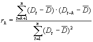
![]()
The part has a seasonal component if r(k) > Limit (k = no of periods per year). The partProfileUpperO2Limit can be changed from Advance Server Settings. Entry SeasonProfiles/partProfileUpperO2Limit. When setting this parameter it can be useful to look at the normal distribution. A value of 1.05 gives 85% accuracy.
When using the automatic season profile the part will have to pass this test to get a seasonal profile computed and used in the forecast making.
A part needs to be above the upper limit to get a seasonal profile, but once the part has used a profile in the forecast making it will need to get a r(k) below the lower limit number to loose the profile. With this no mans land interval will make the forecasting more stabile for parts that are on the limit of getting and not getting a seasonal profile.
Matching of Profiles
Testing whether two seasonal profiles can be matched proceeds like this: P1 and P2 are the seasonal profiles. The two profiles are combined for a two-year-long demand array, then the autocorrelation factor is taken at lag N (N is the number of periods per year). Then this factor is compared to the MLimit. If the factor is higher then the two profiles match; if it is lower then there is no match. The matchLimit can be changed from Advance Server Settings. Entry SeasonProfiles/matchLimit.
![]()
It is also possible to set the minimum number of demand periods a part must have to be considered by the algorithms. This is also done from Advance Server Settings. Entry SeasonProfiles/PeriodsLimit. The last parameter that can be set in Advance Server Settings is the minmum number of parts a resulting profile must contain. This is to prevent an automatic profile generation run from creating many profiles that contain only one part. Entry SeasonProfiles/NumberLimit.
When performing best fit seasonal profile search, the profile with the highest Mlimit wins the contents and becomes the best matching profile for the current part. If Mlimit is negative for all profiles then no profile is set as best fit for that part.
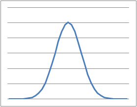
Gauss Filter (Blur)
The Gauss filter smoothes the peaks of a season profile. The graph below shows a typical shape of a Gauss filter. This function can be ran several times the season profile will then become more and more smooth.
![]()
a is a alpha value that will vary with the period version used.
If the period version is under 10 periods per year a=3
All other period version lengths
a= (-0.002537136 * number of periods per year) + 0.931143734
If this gets below 0.005 then a is set to be 0.005.
X is the period number of the seasonal profile.
Applying seasonal Profiles
Applying a seasonal profile on a part is done with the following algorithm (simplified).
1. Remove the seasonality from the parts original history. This is done with dividing by the seasonal indexes. Note that for this we use the parts automatically generated seasonal profile for this (algorithm for this is found here). Then this historical demand is normalized, done by multiplying all periods with a factor = sum(original history/sum(removed history). Then this history normalized history is divided with the average of the seasonal indexes used to remove the seasonality from the original history. Note there is a possibility to set how small this average is allowed to get (see Advance Server Settings).
2. Then the selected forecast model is computed on the resulting cleansed historical demand. (see Forecast models for details). Note that the cleansed demand resulting from point 1 is not shown any where in the graph or tables in Demand Planning.
3. Then the selected seasonal profile is applied to the forecast from point 2. This is done by multiplying by the indexes.