IPR Models
General
The results of an IPR calculation is how much should we order of a SKU when ordering (Lot Size), how much should we have as a buffer stock to have the wanted service (Safety Stock) and finally at when inventory level should an order be placed (Order Point).
Note that there exists 2 parameters called Max Order Cover Time and Max Safety Stock Cover Time these parameters are set in the planning hierarchy and is used to limit the Lot Size and the Safety Stock so that they does not get extremely large. These are especially useful when using the EOQ model since cheep parts can get real high order quantities (can cover many years is some cases). The same goes for service level controlled safety stock where unnaturally high transactions that are not marked as abnormal will result in high safety stocks. These 2 fields will prevent the Lost Size and Safety Stocks computed to be bigger than the number of days that you specify in these fields. This makes these models more robust and safe to use.
There are also 2 parameters that can be set on inventory part called Min Presentation Qty and Max Capacity Qty. The Min Presentation Qty will if set be a floor for how low the Safety Stock can get on a part if the model returns a higher Safety Stock than the Min Qty then the higher Safety Stock value will be used as Safety Stock. The Max Capacity Qty will from a maximum amount of units that will be planned to have on stock after receiving parts, this mean that (Safety Stock + Order Qty) <= Max Capacity Qty. Note there is no guarantee that your Qty on hand never will exceed the Max Capacity Qty this will depend upon the demand during lead time if this lower that anticipated you will exceed the Max. But you plan not to exceed it. There is a field in on the part and in the planning hierarchy where it can be set if IPR should consider the max capacity setting when computing the resutls or not. The reason for setting the Max and not conisder it when computing can be that you onyl wnat to warn the reciving site about the fact that a part will exceed its max limit but still send the IPR computed qty.
If you have a delivery route connected to the part beeing computed, IPR will use information from the route and lead times in the supply chain matrix as the parts lead time and cycle time when planning the purchase parameteres.
IPR can be used on parts with planning method B where the models are explained below. IPR can also be used for parts with planning methods A, D, E, F, G and M it will then compute the safety stock only, and the result is written to the Safety Stock field of the inventory part or in the Time Phased Safety Strock tab on Inventory Part/Planning Data/General(Time Phased Safety Stock). See IPR Time Phased Safety Strock for details.
To determine this there are 4 different models/parameters that needs to be set
- Demand Model
- Safety Stock Model
- Order Quantity Model
- Order Point Model
The Demand model determines where to look for the future demand, this model has 3 settings:
Demand Model
Safety Stock Model
Lot Size Model
Order Point Model
- Manual
- Lead Time Driven
- Slow Movers Life Cycle
- Slow Movers Lead Time
- Croston Life Cycle
- Croston Lead Time
Note that you can see all the detailed calculations in an excel sheet, if you access the IPR server web page <http:://<IPR/DP_SERVER_MACHINE_NAME>:<IPR/DP_SERVER_PORT_NUMBER>/ipr/> e.g. "http:://inmino1:5010/ipr/". Simply type the address in your web browser.
Demand Model - Yearly Prediction
This settings simply uses the field on Inventory Part called Pred Year Cons Qty as the yearly demand for the part. Also a manual set yearly consumption.
Demand Model - History
Uses the Lead Time, Cycle Time, No of Issues in Lead Time and the Avg. Qty per Issue to compute the yearly demand.
![]()
If you look in the inventory part (Planning Data/Order Point) you will se the yearly result in the field Estimated Yearly Demand. Using this setting will be like a simple level forecast model.
Demand Model - Forecast
The future demand is fetched from the forecast from Demand Planning. The forecast will be read from this forecast in given intervals (depending on the models).
Safety Stock - Manual
Uses the manual safety stock set in the Safety Stock field on Inventory Part.
Safety Stock - Time Coverage
When Time Coverage is used the safety stock is determined based on the Safety Stock Cover Time and the Demand Model. The Safety Stock should cover the amount of days demand determined by the two. Example is you have Yearly Prediction as demand model with a yearly demand of 876 and you have 25 as Safety Stock Cover Time this will give a safety stock of (876/365*25) 60.
When forecast is selected as Demand Model. The safety stock is calculated based the forecast in the interval shown below

Safety Stock - Historical Uncertainty
Historical uncertainty uses the measured Standard Derivation in Lead Time together with the Service Rate compute the Safety Stock. The Service rate is the demand you have for the service level over the parts life cycle and the standard derivation states the variation of the demand during the lead time. The Standard Derivation is computed by the Analyze Demand Derivation background job in IFS.
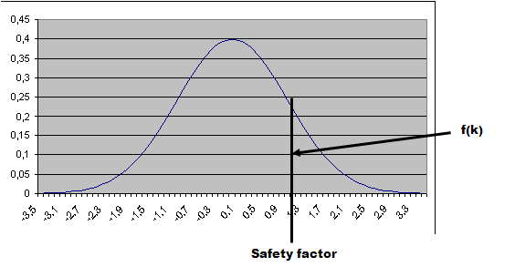
We have the standard derivation measured in the lead time based on historical observations from the Analyze Demand Derivation job. The first step in finding the appropriate safety factor for any given service percentage is to compute the value of the service function f(k).

| OQ | Order Quantity (Lot Size) |
| SD | Standard Derivation |
| SL | Service Demand (0 - 0.999999) |

Notice that as the lot size increases the need for safety stock becomes less and less. The same yelds id the standard derivation decreases.
To find the right safety factor for a given service function we can use the following table
| Safety factor | Service function |
| 0,00 | 0,3989 |
| 0,60 | 0,1687 |
| 1,20 | 0,0561 |
| 1,80 | 0,0143 |
| 2,40 | 0,0027 |
| 3,00 | 0,0004 |
Finally the safety stock is calculated by:
![]()
| SD | Standard Derivation |
| SS | Safety Stock |
Note that the Standard Derivation will be altered when the Dynamic Coverage model is used see Dynamic Coverage.
Safety Stock - Mean Absoulte Error
This method is similar as the Historical Uncertainty with the important difference that the Standard Derivation in Lead Time is fetched from the forecast in Demand Planning and used together with the Service Rate compute the Safety Stock. The Service rate is the demand you have for the service level over the parts life cycle and the standard derivation states the variation of the demand during the lead time. The Standard Derivation is computed from the MSE error for the lead time (plus eventual cycle time) from Demand Planning it is measured one lead time into the future when calculated (se figure).

We have the standard derivation measured in the lead time based on historical observations from the Analyze Demand Derivation job. The first step in finding the appropriate safety factor for any given service percentage is to compute the value of the service function f(k).

| OQ | Order Quantity (Lot Size) |
| SD | Standard Derivation |
| SL | Service Demand (0 - 0.999999) |

Notice that as the lot size increases the need for safety stock becomes less and less. The same yields id the standard derivation decreases.
To find the right safety factor for a given service function we can use the following table
| Safety factor | Service function |
| 0,00 | 0,3989 |
| 0,60 | 0,1687 |
| 1,20 | 0,0561 |
| 1,80 | 0,0143 |
| 2,40 | 0,0027 |
| 3,00 | 0,0004 |
Finally the safety stock is calculated by:
![]()
| SD | Standard Derivation |
| SS | Safety Stock |
Note that the Standard Derivation will be altered when the Dynamic Coverage model is used see Dynamic Coverage.
Lot Size Model - Manual
The Lot Size is set manually on the Inventory Part.
Lot Size Model - Time Coverage
When Time Coverage is used the Lot Size is determined based on the Lot Size Cover Time and the Demand Model. The Lot Size should cover the amount of days demand determined by the two. Example is you have Yearly Prediction as demand model with a yearly demand of 365 and you have 15 as Lot Size Cover Time gives a Lot Size of (365/365*15) 15. When Time Coverage is used and Demand Model is set to forecast. The Lot Size is set to cover the forecasted amount from the lead time into the future for the Lot Size Cover Time number of days.

Lot Size Model - EOQ (Economic Lot Size)
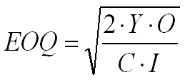
The EOQ balances the cost of ordering with the cost of having the goods on stock and computes the Lot Size so that the sum of the these costs are minimized.

| Y | Expected yearly demand |
| D | First period with historical demand |
| O | Order Cost |
| C | Cost Price |
| I | Inventory Discount Rate |
When you select Forecast as Demand Model we use a special twist to the EOQ model that will take seasonal changes and trends of the foreast into account when computing the Lot Size.
Algorithm
1. By using the forecasted yearly demand Y_0 calculate EOQ_1, starting from the end of lead time
2. Find out how long T_1 EOQ_1 lasts starting from the end of the lead time.
3. Calculate the forecasted demand in the T_1 range, and find the expected yearly demand Y_1 by extrapolation
4. Calculate a new EOQ_(n+1) with Y_1 as yearly demand
Then we repeat from point 2 this is done 3 times, the resulting EOQ_4 is the final EOQ.
Dynamic Coverage
The Dynamic Coverage is a lot size model that uses route id information. The point with this model is that you should get a delivery of parts on each day the part is delivered acording to the route id connected to the part. So based on the route id IPR will compute the latest order day and corresponding delivery day for each delivery day in the route id. The lot size computed should be so that the quantity on hand at the delivery day of the next order is equal to the safety stock. In short if the sale goes as planned you will get and parts delivered each time the part can be delivered acording to the route id info.
The route info will normaly mean that the lead time and cycle time will vary depending on the day of the week, since the standard derivation etc is computed by the Analyse Inventory Part Demand Derivation job in the IFS Inventory module and this job uses the parts Expected Lead Time and the Cycle Time on the part. So the measured standard derivations will be altered with this formula before they are used to compute safety stock.

The lot size is calculated like this:
|
|
Order Day n |
|
|
Receipt/Delivery Day n |
| SS | Safety Stock |
| QTY | Quantity on hand |
| PS | Planned Supply (On..Rn+1) |
![]()
Order Point Model - Manual
The Order Point is set manually on the Inventory Part.
Order Point Model - Lead Time Driven
When Lead Time Driven Order Point is used the Order Point is set to the calculated Safety stock plus the anticipated Demand During Lead time + eventually cycle time. The Demand it will use is decided by the Demand Model. If Safety Stock is 10, lead time is 10 and demand model Yearly Prediction with year qty 730.
The Order Point is 10 + (10*2) = 30
Order Point Model - Slow Moving Life Cycle
When Slow Movers Order Point is used the Order Point is set according to the poisson distribution. NOTE the safety stock is not used in this model this model calculates the Order Point directly. The difference of Lead Time and Life Cycle is that when using Life Cycle you state that the Service Rate is for the parts entire life cycle also called Fill Rate. When Lead Time you set the Service Rate for the Lead Time period only, or 1-service demand is the lowest allowable probability of a storckout in an order cycle.
| OQ | Order Quantity (Lot Size) |
| SD | Standard Derivation |
| SL | Service Demand (0 - 0.999999) |
| R | Order Point/Reorder Level |
| DL | Random demand during lead time |
| λ | Demand rate (daily demand rate) |
The Order point is then calculated by the following algorithm
Step 1. (Bounding Initiation) )k=0
![]()
![]()
Step 2 (Bounding Check) If F(k) > SL then set R1=k and go to Step 4 otherwise go to step 3
Step 3 (Bounding Increment) k=k+1
![]()
![]()
and go to step 2.
Step 4 If OQ=1 then stop R1 is the reorder point. Otherwice go to step 5.
Step 5 (Interation for OQ) Set Rq=R1-OQ

Step 6 (Increase / Decrease decision) If X < SL*OQ then go to Step 7a (keep increasing Rq until X >= SL*OQ else go to Step 8a (keep decreasing Rq until X<SL*OQ
Step 7a (Increasing to reach target)
![]()
![]()
Step 7b (Check) If X>SL*OQ ,then Rq is the desired reorder point. Otherwise go to step 7a
Step 8a (Decreasing to reach target) Rq=Rq-1
![]()
Step 8b (Check) If X<SL*OQ, then Rq+1 is the desired reorder point. Otherwise go to step 8a. In the above steps 8a and 8b are used in case the theoretical lower bound on Rq fails (it happens for small OQ)
Order Point Model - Slow Moving Lead Time
When Slow Movers Order Point is used the Order Point is set according to the poisson distribution. NOTE the safety stock is not used in this model this model calculates the Order Point directly. The difference of Lead Time and Life Cycle is that when using Life Cycle you state that the Service Rate is for the parts entire life cycle also called Fill Rate. When Lead Time you set the Service Rate for the Lead Time period only, or 1-service demand is the lowest allowable probability of a storckout in an order cycle.

| x | The number of occurrences. |
| l | The historical frequency in lead time |
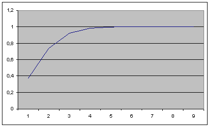
The Poisson distribution gives the probability for 0, 1, 2, 3, 4.. Demand occurrences in the lead time. The occurrences is assumed to be independent. To get the Order point you simply multiply the correct number of demand occurrences with the average demand per occurrence.

| Frequency | Cul. Prob |
| 0 | 0,3678 |
| 1 | 0,7357 |
| 2 | 0,9196 |
| 3 | 0,981 |
| 4 | 0,9963 |
| 5 | 0,994 |
| 6 | 0,9999 |
Frequency λ=1 Avg Issue Qty=2
With a service demand set to 90% this will give a Order Point of 4 (2*2) in the example. This will give a teoretical service during the lead time of 91.96%.
Order Point Model - Croston Life Cycle
This is the same as Slow Moving Life Cycle model with the difference that the frequency is fetched from the Corston forecast model instead of from direct measures of frequencies and demand sizes from historical sales.
These numbers are expressed using the period length selected as the period version of the Demand Planning. For this to make any sense the period version needs to have almost identical period lengths (weeks, months, quarters, or other uniform periods). So when the parts lead time and the period length in Demand Planning is not similar then none of the Croston's slow moving models should be used.
We assume that the lead time is smaller than the forecasted period, we then do a time shift to get the estimated inter arrival time during the lead time (t2), this can be calculated like this.
| z | Demand Size when demand occurs, from Corston's model in Demand Planning (Demand Size) |
| q | The frequency between demand occurrences from Corston's model in Demand Planning (Inter Arrival Time |
| t1 | Average period length in demand planning |
| t2 | Lead time of the part |
![]()
![]()
Then we can estimate the demand size during the lead time t2, this can be calculated like this
![]()
![]()
Then these are used in the same algorithm as for Slow Moving Life Cycle
Order Point Model - Croston Lead Time
This is the same as Slow Moving Lead Time model with the difference that the frequency is fetched from the Corston forecast model instead of from direct measures of frequencies and demand sizes from historical sales.
These numbers are expressed using the period length selected as the period version of the Demand Planning. For this to make any sense the period version needs to have almost identical period lengths (weeks, months, quarters, or other uniform periods). So when the parts lead time and the period length in Demand Planning is not similar then none of the Croston's slow moving models should be used.
We assume that the lead time is smaller than the forecasted period, we then do a time shift to get the estimated inter arrival time during the lead time (t2), this can be calculated like this.
| z | Demand Size when demand occurs, from Corston's model in Demand Planning (Demand Size) |
| q | The frequency between demand occurrences from Corston's model in Demand Planning (Inter Arrival Time |
| t1 | Average period length in demand planning |
| t2 | Lead time of the part |
![]()
![]()
Then we can estimate the demand size during the lead time t2, this can be calculated like this
![]()
![]()
Now we take the 1/q2 and use that as l in the poison distribution. z2 is used as the anticipated demand when we get an occurrence.

The Poisson distribution gives the probability for 0, 1, 2, 3, 4.. Demand occurrences in the lead time. The occurrences is assumed to be independent. To get the Order point you simply multiply the correct number of demand occurrences with the average demand per occurrence (z2).