Constraint Based Scheduling
Introduction
IFS/Constraint-Based Scheduling solves the problem of when to complete a given set of jobs that represent work on a set of resources, e.g., machines, labor (persons) or tools, that can complete this work while attempting to meet some objective. The scheduling problem concerns three elements: to determine at a detailed level which work center, labor or tool resource should do what and when. This means that you must find an optimized assignment of resources to tasks, an optimized order in which the tasks are to be processed and an optimized time when the processing is to be done. There are different types of scheduling. Predictive scheduling makes an optimized schedule from a given set of orders. Reactive scheduling reacts to changes in the schedule and restores it to a usable condition. Interactive scheduling permits the direct manipulation of the schedule.
Scheduling makes use of a production plan to develop a detailed schedule of the work to be done. If planning is about the creation of a scenario that the organization can perform within to reach its objectives, then scheduling is about how to manage the execution of that scenario in the best possible way. Scheduling is based upon a plan, except when using DOP. In that instance, scheduling and DOP planning work together.
The manufacturing system that performs the schedule has constraints that govern its ability to reach the objectives. The constraints are the limitations of the materials needed and the resources (machine, person, tools). The availability of material and resources, the availability of specific resources that can be assigned to a particular operation, and the preference relationships between operations, among others, can be considered as limitations. These must be taken into consideration when constructing the schedule. The objectives for the schedule are often conflicting and not always easy to quantify. This implies that the goal when creating the schedule is to find some sort of trade-off between different objectives and it also implies that some objectives need to be quantified using rough estimates. Within the scheduling domain there are global objectives, e.g., minimized average tardiness for all orders in the schedule or minimized total holding cost. There are also local objectives, e.g., minimize setup for a machine in a given time frame or maximize throughput for a work center. IFS/Constraint Based Scheduling offers alternatives to meet these objectives.
Note: IFS Cloud facilitates infinite scheduling of shop orders. This can be done using the Infinite Scheduler for Shop Orders. For more information, see the topic description on Shop Order Infinite Scheduling. Finite Constraint Based Scheduling is performed using the Advanced Planning Board in IFS Applications.
Advanced Planning Board
Constraint Based Scheduling (CBS) can be performed using the Advanced Planning Board (APB) in IFS Cloud.
The Advanced Planning Board (APB) allows you to perform finite scheduling of shop orders on sites that have enabled the use of the APB in scheduling basic data (referred to as APB enabled sites hereafter).APB only considers the constraints placed by shop orders and resources that are actually loaded to the APB at a given time and not all the shop orders and resources available at the site. It also depends on whether the work centers used for the shop order operations have finite scheduling capacity.
By using the APB, it is possible for a number of users to schedule the
same or overlapping subsets of operations simultaneously. The scheduling process
is supported by a graphical representation of operations, material, work centers,
tools, calendars, and so on. This powerful graphical interface allows you to
work with the schedule interactively. You can move the operations and resources
along a timeline using drag-and-drop and schedule them to meet your requirements.
The changes you make can then be saved back to the database and the changed
shop orders will be updated accordingly.
It should be noted that APB to schedule shop orders at a particular site,
the shop order infinite scheduler is also active for the same site. Therefore
the same subset of shop orders may be scheduled by the infinite scheduler as
well as through the APB. However, only the schedule which was saved last, either
by using the infinite scheduler or the APB, will be valid.
If the latest
schedule was established using the APB, the value in the CBS Scheduled field
of the shop order operation line will be Scheduled. If the latest schedule was
established using the shop order infinite scheduler, the value in the CBS Scheduled
field will be Infinite Scheduled. If an operation has either been parked or
if it has been unscheduled by APB , the value in the CBS Scheduled field for
that operation will be Unscheduled. For instance, when you create a shop order
it will be scheduled by the infinite scheduler first. This order may subsequently
be rescheduled through the APB. As a result, the schedule created by the infinite
scheduler gets replaced. This can happen the other way round as well, when a
shop order schedule which was saved using the APB gets replaced when it is rescheduled
using the shop order infinite scheduler. Changing the site calendar,
for instance, will cause the infinite scheduler to run automatically. Canceling
a machine operation or splitting a shop order are also examples of instances
when orders may be rescheduled by the shop order infinite scheduler.
It should also be noted that the data presented in the APB is not constantly
synchronized with the data in the database. You need to reload data to the APB
to see the latest data from the database at a given time.
As stated previously,
shop orders on APB sites can also be scheduled using the shop order infinite
scheduler. As the name suggests, it performs infinite scheduling on shop order
operations within a site. For more information, see the topic description on
Shop Order Infinite Scheduling.
Planning and Scheduling
A schedule is based upon a production plan. The schedule describes when to complete work on parts while the plan describes what parts to produce and when to produce them. There is one major difference between planning and scheduling. Planning is based on probabilities while scheduling is deterministic. There are no average levels of availability or work to be performed in scheduling. For example, the availability of a resource in scheduling is based on the work time calendar, which can have specific interruptions due to maintenance or some other disturbance, as opposed to planning, where CRP is based on expected average levels of utilization to cover for such interruptions. The reason is obvious. In the near future, an average value of availability is of no use since you have to determine start and finish times for different tasks at a very detailed and accurate level.
The following rules also have to be considered when scheduling;
Work Center Utilization: The utilization is the percentage of effective
work hours per day (out of the total work hours for the day in the work center
calendar). The default value is 100. For example, if utilization is defined
as 50 for a work center which uses an eight hour day calendar (8:00 A.M. to
4:00 P.M.), the effective work hours will be from 8:00 A.M. to 12:00 noon. The
shop order scheduler will schedule a two-hour operation from 8:00 A.M. to 10:00
A.M. if the scheduling direction is forward and from 10:00 A.M. to 12:00 noon
if the scheduling direction is backward. The utilization percentage has no effect
on scheduling if operations are scheduled by the Advanced Planning Board.
Operation Efficiency: The operation efficiency affects only the
run time, not the setup time. When operation efficiency is set to less than
100% (default value) the remaining run time for machine and labor will be increased.
This will result in an increased value for remaining manufacturing hours which
could affect the scheduled start and/or stop date of the operation. When changing
the operation efficiency, the change will also affect the standard cost of the
operation. Changing the operation efficiency can be done on specific operations,
if there is running-in periods for a while, which temporarily will affect the
performance of the operation.
Work Center Resource Efficiency:
The resource efficiency affects both run time and set up time. If the resource
efficiency is less than 100% (default value), the operation will be scheduled
during a longer time period, because the set up and run time will increase.
Only scheduling is affected (start and finish date on the operation), not remaining
manufacturing hours. Changing resource efficiency can be done if there are different
machines (resources) operating in the same work center with different capabilities.
Constraints
The APB constructs schedules that are feasible with respect to the following constraints. Constraints can be divided into relaxable and nonrelaxable. A relaxable constraint is a usually a goal of the system that does not need to be met to provide a feasible schedule. A nonrelaxable constraint cannot be violated, because violating it will make the resulting schedule infeasible.
| Constraints | Description | Type |
| Functional | Limits the types of operations a specific resource can perform. | Nonrelaxable |
| Capacity | Restricts the number of jobs a resource can process at any given time. | Nonrelaxable/Relaxable (dependent on Finite or Infinite scheduling) |
| Availability | Specifies when each resource is available (hours per day). | Nonrelaxable |
| Precedence | Defines the succession between operations. | Nonrelaxable |
| Run time | Specifies the length of time an operation occupies the resource. | Nonrelaxable |
| Setup | Specifies the setting a machine must have in order to process the operation. This setup may be dependent upon the sequence of the parts scheduled for a machine. | Nonrelaxable |
| Latest Possible Start Time (LPST) | Specifies the latest time the job can start in order to keep the need date. | Relaxable |
| Material Availability | Specifies the quantity and date on which a material is available. | Nonrelaxable/Relaxable (dependent on Finite or Infinite availability) |
Parallel Operation Precedence Constraints
If two operations are parallel, it means that they can be done totally independent of each other. The APB scheduling logic tries to schedule them so their output reaches the succeeding operation simultaneously.
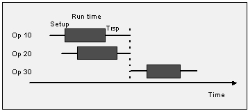
Figure 1 - Operations 10 and 20 are scheduled parallel
Planning Constraints
The need date of orders based upon a material requirements plan is also a constraint. The schedule must be produced without the capability to alter this plan. Changes to the plan can affect the schedule, but the schedule cannot affect the plan. In this way, planning constraints scheduling by not providing the ability to adjust the plan based upon the schedule.
Note that if you are using the condition code feature within IFS Cloud, condition code values are not considered when planning material. That means that no distinction between normal, reworked, repairable, or other conditions on material are made. In addition, any requisitions or orders created by any planning process will be created using the default condition codes specified for the parts. CBS will not try to match the condition of supply material with the condition specified on the demand.
Objective(s)
A shop order can consist of a list of needed materials, and of a chain of operations that should be done in a particular order. The process of making a schedule is constrained by the availability of the materials, the availability of resources at hand, and other logical constraints. To measure how good a schedule is, there are some key metrics such as average tardiness and total holding cost.
There are some key objectives to accomplish when constructing a schedule:
- minimize lead times
- create a feasible schedule with respect to all non-relaxable constraints
- ensure that orders are not started too early, i.e., minimize WIP
- minimize setups
- minimize tardiness
Constructing a Schedule
When constructing a schedule, many different steps are taken using different algorithms. First, material availability and resource assignment options are evaluated. Then, the earliest and latest possible start times for all operations are determined. Based upon a selected priority rule, these time values are used to sort the operations in the order in which they will be scheduled. The operations are then scheduled forward with the finite capacity constraints of the materials and resources. After scheduling, there are some optimization techniques that can be chosen. ALAP moves all operations as close to their need date as possible. Compress Downstream moves operations as close together as possible from left to right. Part characteristic-based sequencing can be used to meet objectives to minimize setup times as well as meet additional constraints based upon part characteristics. All of these algorithms and processes enable the organization to better meet its objectives on the shop floor.
Resource Assignment Strategies
When there are alternative resources, e.g., two resources in a work center, multiple persons and multiple tools, a choice must be made regarding the resources to which the load will be assigned. CBS always chooses the combination of resources that gives the earliest completion date. Additionally, in case more than one infinite resource is available to choose from (e.g Infinite work center has 10 work center resources available), then CBS will give priority to the least loaded resource (in its total life span) when scheduling the operation. This method provides a well distributed load among multiple infinite resources. This load distribution mechanism is enabled for APB when scheduling operations.
Material Availability
A part's availability can be defined as Infinite, Finite (within a specific lead time), or Always Finite. The parts with infinite availability do not constrain the schedule. For parts with finite availability, APB checks for the required amount as it schedules. The required amount can be comprised of an existing supply or from a new supply within the part's lead time. After the part's lead time, APB assumes the part has infinite availability. For parts that always have finite availability, the required amount needs to be available to schedule an operation. As APB schedules, it records the quantity and the date and time at which the material is consumed and produced.
Determine Latest and Earliest Possible Start Times
Determining the latest and earliest possible start times is done using infinite scheduling. This procedure is equivalent to an infinite backward scheduling of all operations.
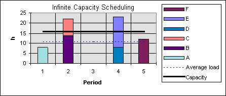
Figure 2 - Infinite capacity scheduling using backward scheduling
Sequence Operation for Scheduling
There are three options for sequencing operations for scheduling a site. These determine the order in which operations are scheduled, which has an effect on the objective(s) of the schedule. The options available are the priority rules First Come First Served, Latest Possible Start Time, and Earliest Due Date.
| Priority Rule | Objective | Sort in Ascending Order of |
| None | Maintain existing sort order | Not Applicable |
| First Come First Served | Complete work in the order it was received | Date Entered |
| LPST | Minimize average tardiness | Latest Possible Start Time |
| Earliest Due Date | Minimize maximum tardiness | Need Date |
Forward Finite Scheduling
Since it is normally impossible to do something in the past, you use forward scheduling as the starting finite scheduling strategy. The scheduling starts from a point in time slightly ahead of the current time, called the global Earliest Possible Start Time.
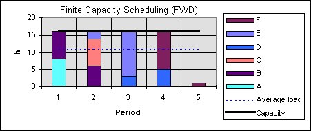
Figure 3 - Finite capacity scheduling using forward scheduling
Forward scheduling means that you schedule the first operation as soon as possible, then the second operation as soon as possible after the first one, etc., until finally, the last operation is scheduled in the same way. With Capacity Constraint scheduling, forward scheduling means as soon as possible when there are materials and resources available. Forward scheduling ensures that the schedule is realistic with respect to all constraints. Forward scheduling means that the scheduled order might not be completed in time. It can also get started unnecessarily early.
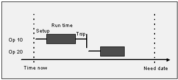
Figure 4 - Forward scheduling starts from the current date with the first operation
There is no way to ensure that every order will be completed on time, since material availability and resource capacity is finite, and you do not schedule anything with a date in the past. When an operation passes its needed time, it is marked as Late. The problem can be solved by increasing the material availability or the resource capacity, or by switching places with another order in the schedule.
As Late as Possible
If you do not want to start the order too early, you can do an As Late as Possible (ALAP) adjustment. This moves all operations as close to their need date as possible, but only if there is free capacity, thus minimizing WIP without breaking any constraints.
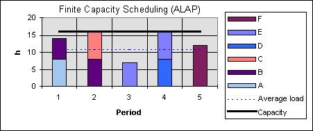
Figure 5 - Finite capacity scheduling using the ALAP adjustment
By performing the ALAP adjustment, no operations start unnecessarily early, thereby minimizing WIP. The bottlenecks automatically set the pace for the preceding operations; due to bottlenecks in the middle of the production flow, there can be unnecessarily long lead times. ALAP accomplishes the same objective as backward scheduling. Backward scheduling is based on the need date. The work has to be completed before a certain date and time. To ensure that the work is scheduled before that date and time, the last task that ends on the need date is scheduled first, then you can proceed with the second to last, etc., until finally, you reach the first operation. This strategy is the most common with infinite scheduling. Backward scheduling ensures that the order is completed on time and that the order is not started too early.
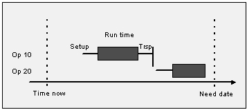
Figure 6 - Backward scheduling starts from the need date of the last operation
Compress Downstream from the Bottleneck
If you want to minimize the WIP in the flow after bottleneck operations, you can perform the Compress Downstream from Bottleneck action. The following graph shows the effect on three orders when WC2 is the bottleneck.
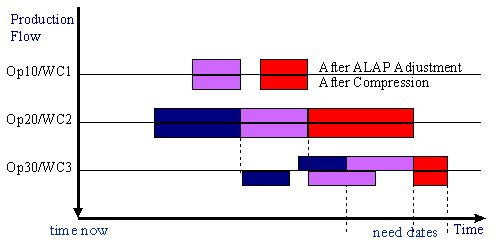
Figure 7 - Compress Downstream from bottleneck
The compress function shifts operations from right to left, closer to their preceding operations. This tends to minimize the processing time for an order and thus reduces WIP.
Part Characteristic-Based Sequencing
With resource-limited scheduling, the overall sequence in which jobs are scheduled into the shop is important for the overall performance. If jobs are scheduled strictly by the LPST dispatch rule then the average tardiness of the schedule should be minimized, but possibly at the expense of setup cost, especially if setups are sequence-dependent. Combining shop orders with the same or similar setup characteristics into batches reduces those costs, but can result in delivery delays. This kind of problem is often present in process-like industries, e.g., printing where the objective is often to sequence jobs, e.g., from light colors to dark. The APB helps you to sequence the shop orders and operations based upon characteristics describing each part. Then it performs sequencing according to part characteristics in ascending/descending order and employing a user-defined time span. This occurs in the same manner as sorting by the various priority rules.