Appendix: HTM Performance
One key aspect of scheduling performance is the time taken to retrieve travel estimates. The PSO solution for estimating travel is to use the HTM database, and this has evolved over time. There is a balance here between accuracy and performance, and some improvements have focussed on performance, while others have concentrated on improved accuracy.
This appendix looks at the impact of the various changes made.
HTM Version History
There have been four significant changes to the use of the HTM since PSO version 6 was first introduced.
- HTM version 1 -> HTM version 2. This change focused on improving HTM performance by changing the way data was stored in the HTM database tables to use more efficient data structures.
- HTM version 2 -> HTM version 3. This change focused on improving HTM accuracy by improving travel calculations over short journeys. This is achieved by calculating the routes for these journeys at run time instead of using pre-calculated values.
- HTM version 3 -> HTM version 4. This change focused on improving HTM performance by improving the efficiency of querying for routing data when calculating short journeys.
- Routing Calculation Mode. This change focused on improving HTM performance by switching the calculation and caching of routing based short journeys to be handled centrally.
As can be seen, most of these changes have been to improve performance. The introduction of routing calculations in version 3 is also optional, so customers who carry out relatively few short journeys can choose not to use this feature if they wish.
Version 2 Improvements
The results below compare performance between using HTM version 1 and HTM version 2, using version 6.2 of PSO.
To measure performance a dataset was sent into the system that contained ten thousand activities. The system was configured to output a plan at regular time intervals, recording the plan margin at each interval. This was repeated for a total of ten test runs so that average results could be determined with good statistical confidence, i.e. to account for the non-deterministic nature of the DSE. See section 'Initial Results' in appendix three for more information on plan margin.
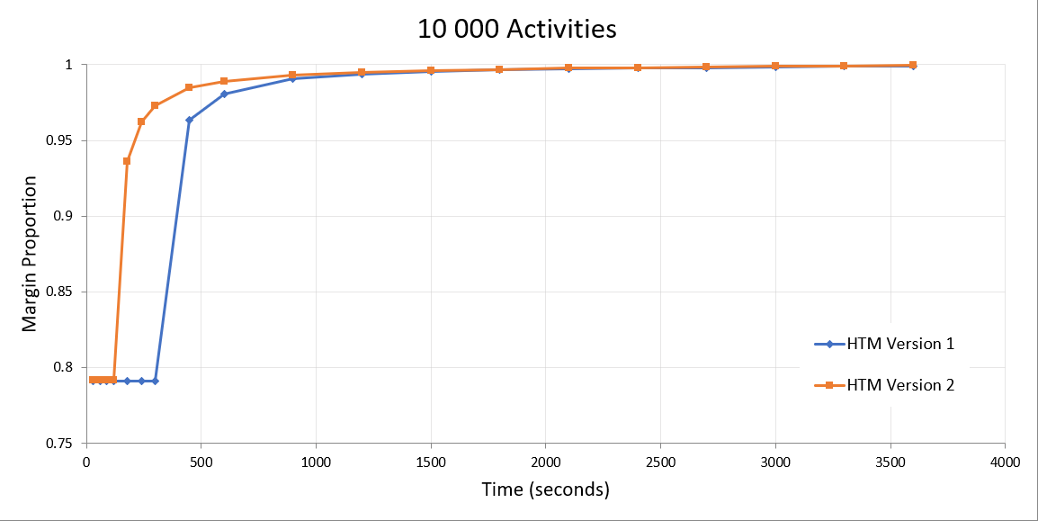
The above graph shows a comparison between using version 1 and version 2 of the GB HD HTM and the difference in the average margin proportion as a function of time. Of note is the time taken for the system to produce the first plan, which corresponds to the "knee" in the curves towards the start of the test run. Also of interest is the time taken for the curve to plateau at the maximum attained plan margin. For both of these measures we see that the Version 2 HTM has improved performance; the time taken to output the first plan is reduced by 60% and the time taken to reach a plan margin proportion of 99% (i.e. 1% off the best value measured) is reduced by 25%. The underlying reason for these differences comes from improved, more efficient data structures in the Version 2 HTM.
Version 2 has a significant improvement of 60% in the time taken for the first plan to be broadcast. Additionally, there is a 25% improvement in the time taken for the system to reach a plan margin proportion of 99%. This is due to an improvement in the efficiency of the data structure used in version 2, leading to a decrease in the time taken to initialize the HTM.
Routing Calculation Mode
This section details the results from a performance analysis of the routing calculation mode.
Scheduling Performance Tests
One dataset was loaded into the system with 15000 activities. The schedule was ran for an hour and was performed ten times, providing a sufficient sample size to allow averaged results to be used with statistical uncertainties in the region of 5% or less.
The RoutingCalculator parameter was altered to allow comparing the following situations:
- InProcess: The individual services that need routing calculations load and process the routing data in the same service.
- TravelAnalyser (Cold Cache): The Scheduling Travel Analyser service handles routing calculations. The Scheduling Travel Analyser service has not already loaded the routing data loaded when the LOAD is sent to the system. This shows the performance of the scheduling when the system has just been started.
- TravelAnalyser (Warm Cache): The Scheduling Travel Analyser service handles routing calculations. The Scheduling Travel Analyser service has already previously loaded the routing data when the LOAD is sent to the system. This shows the performance of the system on following days after previous LOADS into the system have already been processed.
Scheduling Performance Results - Margin Proportion
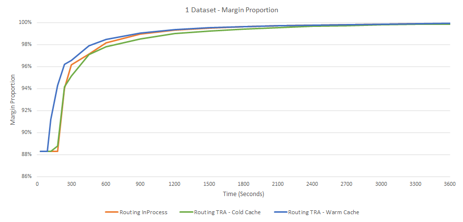
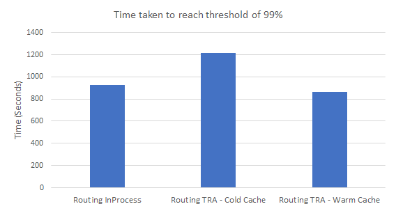
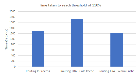
As can be seen from the above graphs there is not a significant change in the plan margin performance by sending the routing requests to the Scheduling Travel Analyser service for processing. When working with a warm cache the initial plans can be generated slightly faster than running InProcess or with a cold cache.
Scheduling Performance Results - Travel Duration Proportion
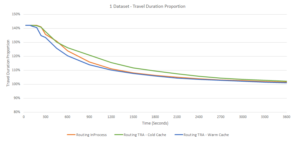
As can be seen from the above graphs there is not a significant change in travel duration performance by sending the routing requests to the Scheduling Travel Analyser service for processing.
Resource Usage Tests
The following charts show the resource usage of the system while processing a LOAD followed by appointment booking.
A dataset with 10000 activities distributed across Germany was sent into a system connected to a vCore Serverless V3 EUR HTM configured with a maximum cores of 4. The first initial 15-20 minutes are spent processing the LOAD and then the following time is spent doing appointment booking at a rate of around one appointment every 6 seconds.
- InProcess: Appointments were returned with a mean response time of 2.9 seconds and a median of 1.8 seconds. The full round trip time was less than 5 seconds for 87% of the requests sent.
- TravelAnalyser (With a warm cache): Appointments were returned with a mean response time of 2.0 seconds and a median of 1.6 seconds. The full round trip time was less than 5 seconds for 97% of the requests sent.
Resource Usage - CPU Usage
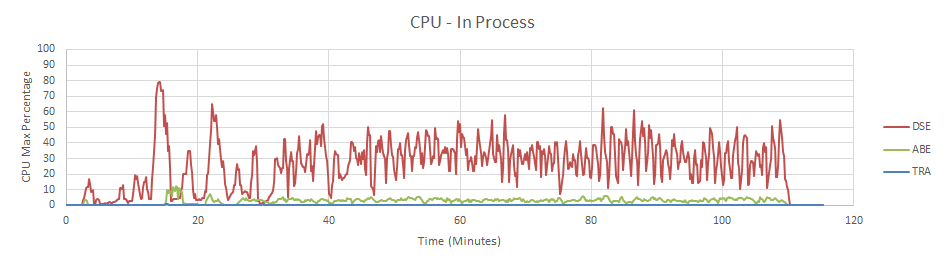
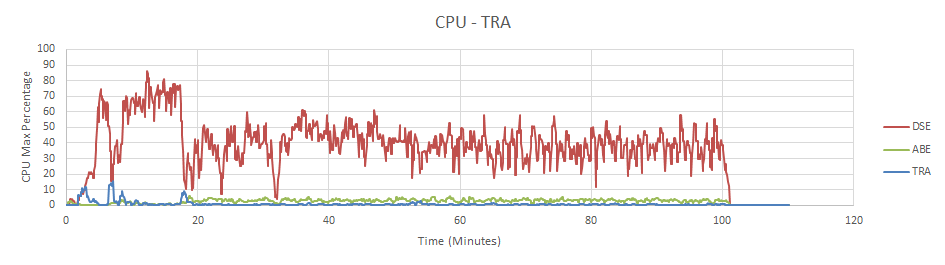
The CPU usage graphs show there is some difference during the processing of the LOAD. When the routing data is already loaded the processing of the travel calculations is quicker. This allows the DSE to spend additional time on scheduling. The line for the TRA service shows where CPU usage has moved from the ABE and DSE into the TRA. During the appointment booking section of the graphs there is very little difference.
Resource Usage - Memory Usage
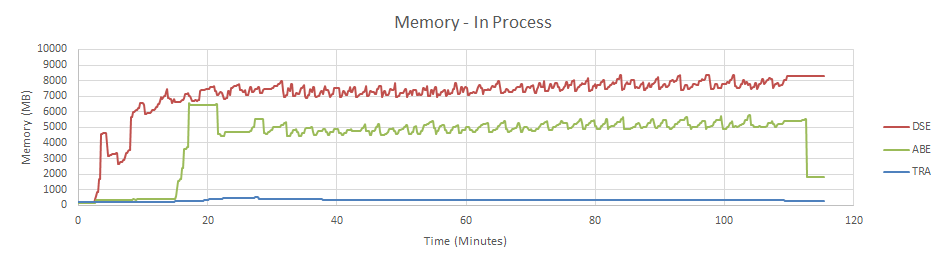
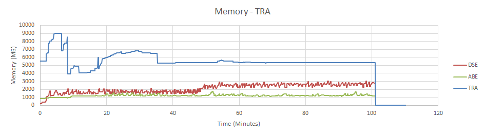
The memory usage graphs show that the overall memory usage of the system is less when the routing calculation mode is TravelAnalyser. InProcess: ~13GB vs TravelAnalyser: ~9.5Gb. These savings will be even greater when multiple ABEs and DSEs are required on a system. This will allow the services to scale up easier.
Resource Usage - HTM Usage
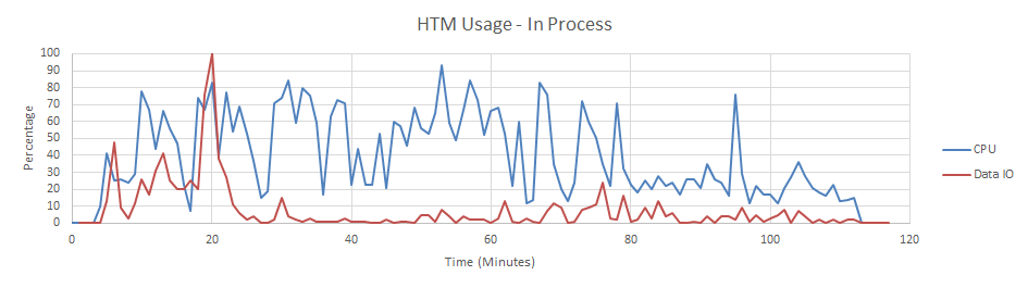
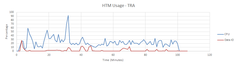
The HTM usage graphs show that the HTM database is used much less when the routing calculation mode is TravelAnalyser. This is especially true for Data IO which is need when loading many routing areas. This is due to two reasons:
- Rather than both the ABE and the DSE making requests to the HTM database to load the routing data only the TRA needs to make requests.
- The TRA can cache the data across LOADs. If a routing area has already been loaded by the previous day then it will still be memory.
Conclusions
Switching the RoutingCalculator to TravelAnalyser has the following benefits.
- Significant reduction in overall system memory usage allowing better scaling when a system has multiple ABEs or DSEs.
- A reduction in the overall usage of the HTM database.
- Initial plans for a LOAD can be generated faster if the routing data has already been loaded (Warm cache).