Appendix: Performance Metrics
In this appendix we present the results of performance tests for specific types of scheduling.
Dynamic Scheduling Performance
Performance comparisons for dynamic scheduling are carried out with every new update of the software, to ensure that there is no regression, and to measure any improvements.
Standard Test Method
The standard test uses an automatically created dataset based in the UK. This is intended to represent a typical service management type scheduling problem:
- There are 10,000 activities at different locations around the UK.
- There are 361 resources each working 5 8-hour shifts.
- The activities range in duration from 20 minutes to 1 hour.
- The activities have a range of values and SLA deadlines.
- There is a basic skill constraint involving two types of skill.
Note
The test data has deliberately been kept relatively simple to allow a clean analysis of basic scheduling performance. As such, the data does not include features such as parts, split activities and activity groups. Tests using different input data are also performed as and when required to check performance when using specific types of functionality, and different sizes of data.
PSO was installed on a standard Azure environment using the latest standard D series machines. The environment consisted of 1 DSE server and 1 IO server, each with 8 allocated cores. In each test, a dataset was sent to the PSO system with broadcasts configured to output statistics of interest at regular intervals over a period of an hour. A total of 10 test runs are performed on each version so as to allow averaged results to be calculated - this is a necessary step when using a non-deterministic algorithm such as the DSE. The test data used is of process type 'dynamic'. Tests are performed with the latest UK HTM.
Further to this, at the end of each test run, a change file was sent in to advance the current schedule time to five minutes into the start of the shifts. For this stage of the test, the broadcasts were configured to output statistics over the next five minutes.
Latest Version Comparison
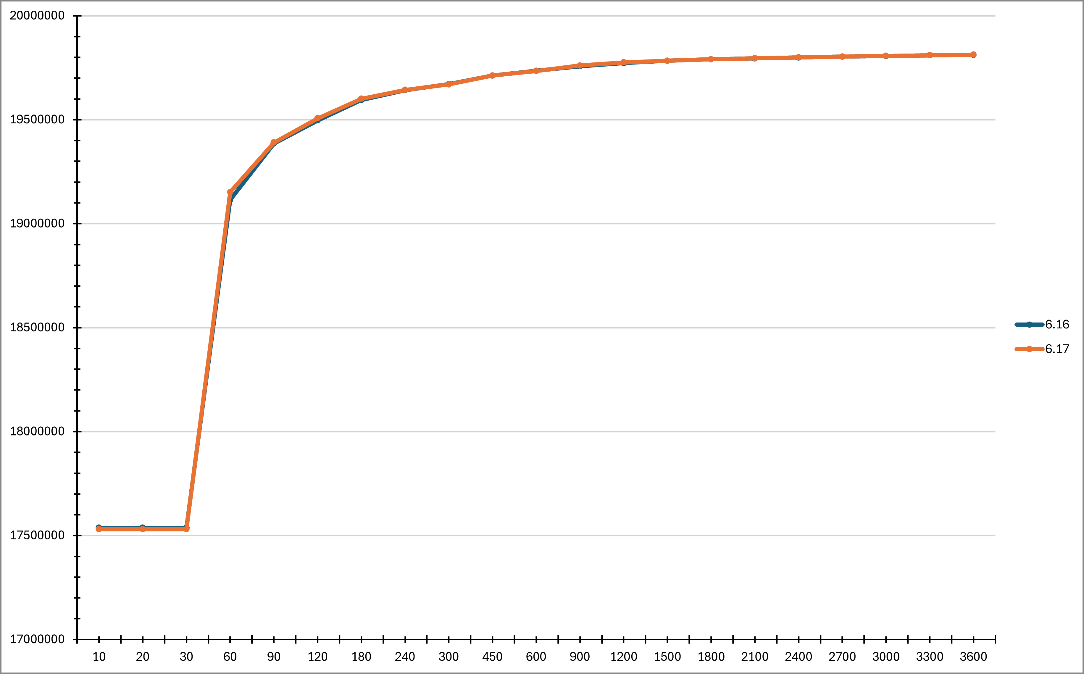
The results from a performance comparison between versions 6.16 and 6.17 are shown in the above figure. The tests used a dataset of 10,000 activities and the latest V4 GB HTM, with each curve representing an average of 10 test batches to reduce variance. The figure indicates that the performance of 6.17 is comparable to 6.16, showing similar times to produce an initial plan and comparable improvements to the plan margin during the early stages of optimisation.
Performance Improvements
The details below document notable performance improvements that have been seen over previous versions:
Version 6.13
In version 6.13 improvements have been made to handling unallocated activities on updates. This significantly improves the performance for schedules with many unallocated activities, and especially when using the APPOINTMENT process type. There is also a general improvement in performance as evidenced by the version comparison using the standard performance test data.
The graph below shows a performance comparison using a 30,000 activity schedule over 30 days using process type APPOINTMENT. This included 1,000 reactive activities that needed to be done within the first few days, 5,000 appointed activities that needed to be done on a specific day, and 24,000 maintenance activities that could be done over a wider availability window.
There is a noticeable improvement in the time taken to produce an initial plan in the 6.13 version, and a subsequent increased plan margin as the schedule improves.
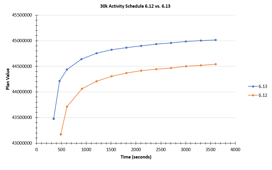
Furthermore, the time taken to process a change was also greatly reduced in the 6.13 version. This was tested using a change to shift the timeline forward by 5 minutes. The 6.12 version took 2.5 minutes to produce a first plan after the change was sent, but this was reduced to less than 40 seconds in the 6.13 version.
Version 6.8
In version 6.8 a small improvement in performance when the HTM was used. This can be attributed to an improvement in the time taken to fetch the initial travel estimates from the HTM.
Version 6.5
In version 6.5 an improvement was detected in the time taken for the DSE to produce an initial plan when using an equivalent HTM.
Version 6.4
In version 6.4 significant improvements were made to the performance when scheduling high density problems, and problems with high volumes of fixed time activities. The 6.4 version could achieve a plan margin in 2 minutes that it would take 15-30 minutes to achieve on the previous version.
Version 6.2
In version 6.2 a significant improvement in performance was detected. The time taken for the plan margin to reach 99% of its final value was reduced by around 40%. The DSE also responded significantly quicker to a change being made to the schedule.
Appointment Booking Performance
In this section we present the results from a performance analysis of appointment booking within PSO. This involves 3 tests based on 2 sets of data.
Dataset 1 - Germany
The load data used for this test was automatically generated test data, designed to represent a typical appointment booking dataset. The data contained the following:
- 11,500 call type activities, of which:
- 10,000 were restricted to a half-day 'appointment' slot, to represent previously booked appointments.
- 1,500 were high priority reactive calls
- 250 resources, each with shifts spanning an 8 week period, and including a one hour lunch break.
- All calls and resources were located in Germany.
Appointments were then requested for 2 slots per day (AM and PM) over a 1 week period, a total of 10 slots for each request. A total of 1000 requests were sent with 1 every 5 seconds. All appointment requests were non-blocking. Provided that an available offer was returned, the activity was then updated to be restricted to the selected slot, and subsequently scheduled by the DSE.
Dataset 2 - USA
This uses a larger dataset containing around 32,000 activities, and 3,000 resources, based in the USA. The test uses a 2 day scheduling window which extends to 2 weeks including the appointment window.
Appointments were then requested for 6 slots per day over a 5 day period, a total of 30 slots for each request. A total of 1000 requests were sent. Provided that an available offer was returned, the activity was then updated to be restricted to the selected slot, and subsequently scheduled by the DSE.
Appointment requests were sent at 2 different rates, firstly at an average of 1 every 2 seconds, and secondly at 2 requests per second. All appointment requests were non-blocking. For the second test an appointment fallback profile was used. This means that the engine initially uses a straight line travel estimate when evaluating slots for any travel estimates that are not already cached. The HTM travel estimate is always used when confirming the accepted slot.
Environment
The test was carried out using a standard PSO Azure system set-up with two 4-core servers, one hosting a single DSE component and the other hosting all other required components. The DSE and Appointment Booking Engine were connected to the latest HTM (Europe / North America depending on the data). The tool used to carry out the test was hosted locally, so all requests were sent from a local server to the Azure system.
Results
| Dataset | Request Rate | Average Offer Response Time | Average Full Round Trip Time | Sub-Second Round Trips | Available Offers |
|---|---|---|---|---|---|
| Germany | 12 per minute | 0.32 seconds | 0.47 seconds | 96.8% | 97.9% |
| USA | 30 per minute | 0.38 seconds | 0.51 seconds | 93.6% | 98.0% |
| USA | 2 per second (with fallback) | 0.83 seconds | 0.98 seconds | 52.6% | 98.2% |
The full round trip time records from when the test tool starts to send the request to when it has received the response. The offer response time is until the appointment booking engine had produced a response.
In all cases there was at least one available slot for every request. Thus, all requests were successfully appointed.
These results have been updated for the 6.18.4 release version.
Note
See the appointment booking guide for further details of the options that can be used with appointment booking, including the appointment booking fallback functionality.
Cyclic Scheduling Performance
In this section we present the results from a performance analysis of the cyclic scheduling mechanism available within PSO.
Data
The load data used for the test was automatically generated test data, designed to represent a typical large cyclic scheduling dataset. The data contained the following:
8,000 repeatable call type activities, each linked to a modelling pattern to govern the required repeat rate:
- 4,000 were required to be carried out once per week.
- 750 were required to be carried out twice per week.
- 700 were required to be carried out three times per week.
- 600 were required to be carried out once per day (i.e. 5 times per week).
- 850 were required to be carried out once every two weeks.
- 600 were required to be carried out once every four weeks.
- 500 were required to be carried out once every 12 weeks.
This results in around 250,000 possible visits, though due to the limited number of resources it was only possible to schedule around 200,000 of these visits.
200 resources, each with shifts spanning a 24 week period.
- All calls and resources were located in Germany.
Environment
The test was carried out using a single 8-core server, with the DSE connected to the latest European HTM.
Method
This data was sent to the DSE for scheduling using each of the following time limits: 1 hour, 2 hour, 3 hour, 5 hour and 15 hour (representing an overnight run). Each time limit was tested 3 times and the results below are an average across the three test runs.
In addition, a standard scheduling dataset was created with equivalent data but using pre-requisites to link the visits together, and the standard 'DYNAMIC' process type.
Results
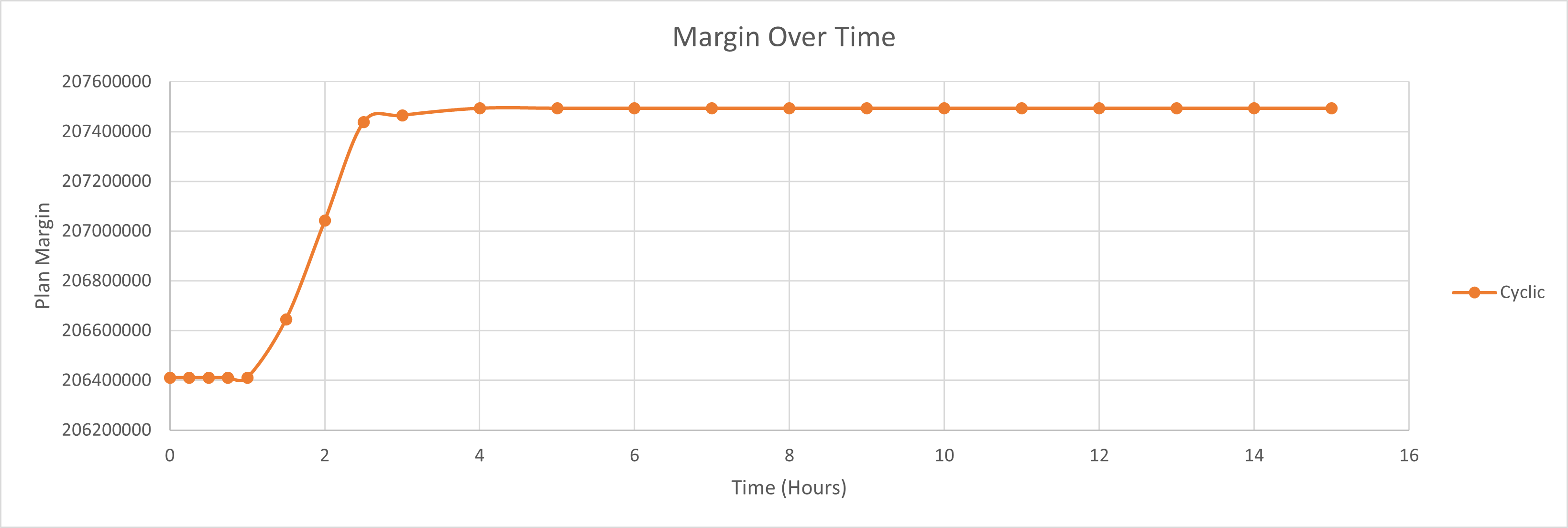
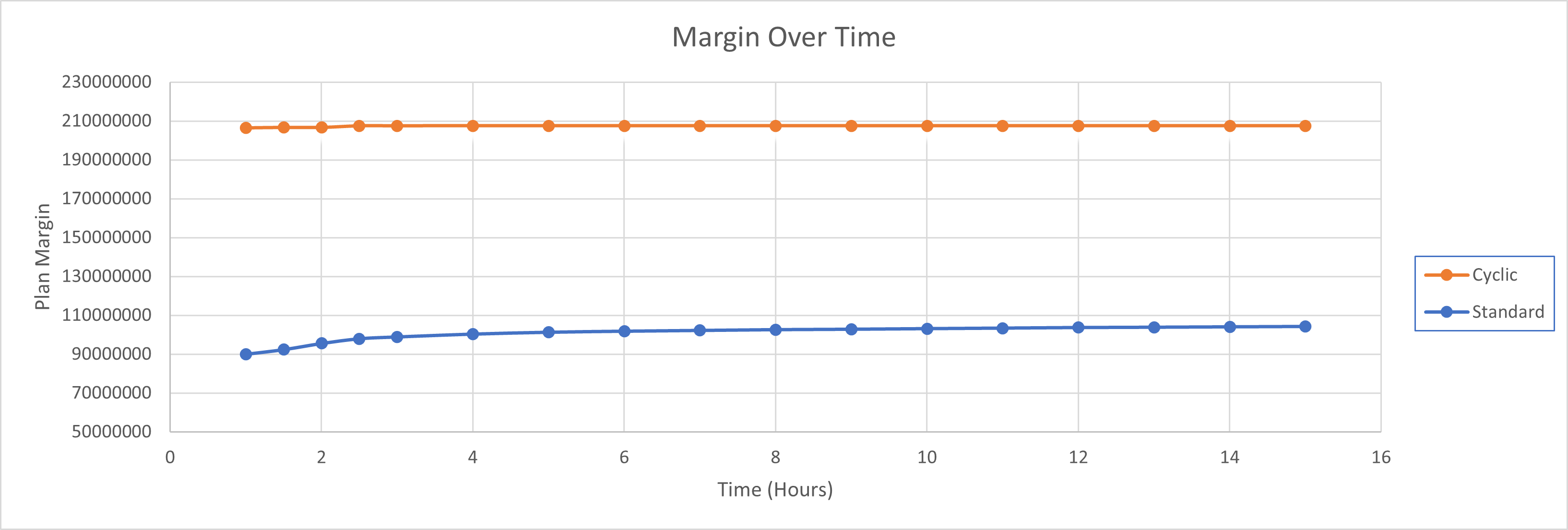
The graphs below show the results of this testing. For the cyclic scheduling runs, there was some improvement shown with each increase in time limit, though the rate of increase reduced considerably after the 3 hour mark. Tests were also carried out where the dataset was allowed to run for longer than 15 hours and there was no measurable improvement beyond this point.
All cyclic runs produced significantly better results than the equivalent standard scheduling problem, showing the benefits of the cyclic approach.
These results were first recorded using the 6.4 version of the product and have since been repeated with the 6.11 release, which yielded an improvement in cyclic scheduling performance.
WISE Performance
In this section we present the results from a performance analysis of the DSE scheduling WISE problems.
Data
The load data used for the test was automatically generated test data, designed to represent a typical WISE problem. Three versions of the data were created, with a total of 5,000 activities, 10,000 activities and 15,000 activities respectively.
In each dataset 20% of the calls were higher value activities with a 1/2 day window of availability, and 80% were lower value with full availability. There were also 20 urgent activities in each dataset.
In addition, 25% of the activities required an 'advanced' skill that only 20% of the resources possessed (these resources were able to carry out all activities).
Each dataset included one resource for every 50 activities (i.e. 100 resources in the smallest dataset, and 300 in the largest). Each resource had a week of shifts, and was able to carry out around 6-7 activities per day, meaning that the initial resourcing was able to carry out around 60-70% of the work.
3 options were available to the DSE to adapt the resourcing:
- Add a new 'basic' resource, with a cost of 5,000 (equivalent to 10 low value activities).
- Add a new 'advanced' resource, with a cost of 10,000.
- Transition a basic resource to an advanced resource, at a cost of 3,000.
Finally, the DSE was given a target that at least 95% of the work should be allocated.
Environment
The test was carried out using a 4-core server, with the DSE connected to the latest European HTM.
Method
Each dataset was run 10 times with each run lasting for a total duration of 1 hour. Results were also captured at intermediate times. The results below are averaged across the 10 runs.
Results
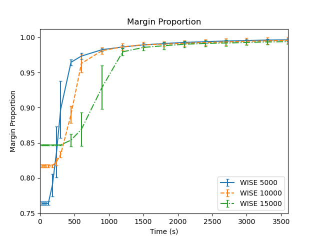
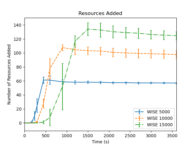
The results show that in each case the DSE was able to allocate almost all of the activities in the schedule (for the final few activities it is not cost efficient to bring in additional resources). As expected this occurs faster on the smaller dataset, but even on the 15,000 dataset the DSE reaches this level well before the full hour has elapsed.
The table below shows how the percentage of resources added in each case is actually slightly lower than the percentage of additional activities allocated. The primary reason for this is likely to be that the WISE is better able to target areas where additional resourcing is required, resulting in a more evenly distributed workforce than in the original data.
| Total Activities | Initial Activities Scheduled | Final Activities Scheduled | % Increase Activities Scheduled | Initial Resource Count | Final Resource Count | % Increase Resource Count |
|---|---|---|---|---|---|---|
| 5000 | 3069 | 4932 | 60.7% | 100 | 157 | 57% |
| 10000 | 6653 | 9958 | 49.7% | 200 | 297.6 | 48.8% |
| 15000 | 10812 | 14944 | 38.2% | 300 | 424.6 | 41.5% |
The effect of running for additional time can be seen in the shortening of the error bars in graphs below. This shows that with more time the DSE will arrive at a more consistent result. In each dataset after the full hour the number of added resources was within 6% of the average recorded value on every run. The DSE also transitioned a small number of existing resources from basic to advanced in each case - around 0.1% of the existing workforce.
Comparison of Results to Previous Versions
A comparison of tests on the current and previous versions (6.7 and 6.6, respectively) shows no significant difference in the results.