Travel In Scheduling
What is travel in scheduling?
A travel is the duration and distance needed for a resource to go from one location to another. For example, on a typical work day (shift) a resource may need to travel from his/her home location to a set of locations to undertake activities the resource has been assigned. This will most probably require the resource to travel for a certain amount of time in his/her shift.
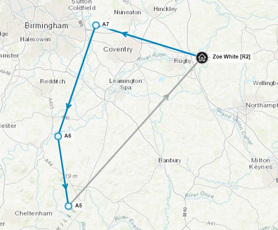
The light blue lines on the map below represent a resource's expected travel between each of the resource's assigned activities today (on the Mapping tab):
The dark grey lines below on the resources' timeline represent a resource's expected travel between all the resource's activities today:

The orange coloured activity represents an activity to which the resource is currently travelling towards:

The DSE's scheduling algorithm is score-based, i.e. activities scheduled to resources have a value to be done and travels the resource needs to make have a cost. Hence, the DSE requires to know the duration of this travel to factor the travel cost into its decision making. By having this knowledge, the DSE can decide what is the optimal way the resource can go about doing these jobs/activities by minimising travel where possible.
Note
There are usually other constraints the DSE needs to obey, such as time constraints or missing skills or parts, so that the route it produces is not always the 'least possible travel' route.
Each time the DSE is attempting to produce a new schedule it needs to know all the combinations of travels possible between the resource home locations and all the activities (including travels between the activities). This may be a very large number of travels depending on the size of the schedule. Hence, attempting to get the travels from a routing engine API or something similar is not a solution since it would slow down the plan generation of the DSE significantly. The various travel source options are outlined in the next section.
Note
Note that the schedule is usually clustered, so that the DSE will only require travels within a cluster at any point in time, which reduces the amount of travels needed slightly.
Travel Options
There are three ways to obtain travels:
- HTM: a database of pre-calculated travels between nodes in the area covered by the schedule. Travels are calculated based on routing data from Tom Tom. The HTM database is highly recommended for Scheduling implementations as it provides a quick way of getting travels that model the real world accurately. Road network routing can be used for short travels where a higher accuracy is required.
- Straight Line: 'as the crow flies' travel calculation that has no knowledge of the road network. Not recommended for live scheduling environments.
- Real Time Travels: the DSE may be configured to use real time travel information from online routing services for certain journeys. This includes up-to-date traffic information and possible road closures.
Hierarchical Travel Matrix
The HTM database is a read-only database that is used by Scheduling services, whenever travels are needed for their functionality. There are four Scheduling Services that use the HTM to get travels:
- Dynamic Scheduling Engine: gets the travels it needs from the HTM database in order to optimise the ordering of the activities in geographic routes by minimising travel.
- Appointment Booking Engine: uses the travels in a similar way to the DSE.
- Scheduling Travel Analyser: uses the HTM to get travels used to calculate isochrones.
- Scheduling Workbench: uses the HTM in the Schedule Assist tab on the Scheduling Workspace.
The HTM is mainly used to get travels between locations in the scheduling input, i.e. activity and resource locations, so that the DSE or the ABE can make a sensible decision on the sequence of activities within a shift. The advantage of using the HTM is two-fold:
- speed: it is more efficient to get travels using the HTM rather than getting travels from a routing engine API over the web. Remember the DSE may require hundrends of thousands of travels to make a scheduling decision at any time - depending on the size of the scheduling problem of course.
- accuracy: it is a lot more accurate to get travels using the HTM, mainly because it has a knowledge of the routing network - data sourced from routing data provider Tom Tom - and it has various levels of accuracy depending on the distance between the locations a travel is requested for.
The HTM is defined as a layered travel matrix of travels between pre-defined nodes. A normal HTM typically contains 3-4 hierarchy levels, where each level is defined by its node density, i.e. the distance between all its nodes.
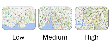
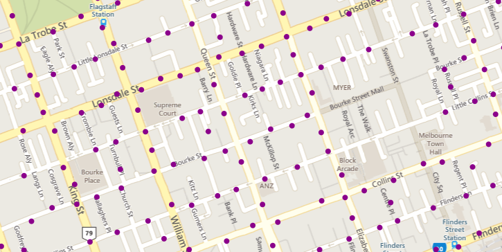
The nodes are chosen by setting up a grid of equal distance nodes on the map and then snapping these nodes intelligently onto the road network (taking into consideration for example whether the node snapped is a junction).
The HTM doesn't have a travel from one node to all the other nodes in each hierarchy level in the matrix - to reduce the size of the database. Only the lowest density hierarchy level has a travel to each of the nodes in the level, where nodes could be 4-5km apart from each other. In all the other hierarchy levels travels are calculated between nodes within a certain radius. The value of this radius depends on the density of the nodes. 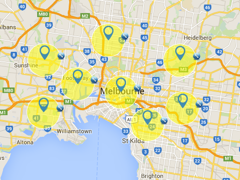
Note
The timings for boat and ferry routes is not known when generating an HTM, so the journey time for a boat/ferry route is estimated. This estimate is usually fairly pessimistic so as not to schedule a journey that cannot actually be completed in time.
Routing
Note
Routing requires at least a V3 HTM.
Some scheduling problems have a particularly high number of activities in very close proximity, e.g. in a small area of a city centre. For these scheduling problems the pre-calculated HTM travels may not be sufficient as the nodes are not dense enough. In these cases a routing calculation using the road network can be used.
The below image shows an example of a travel. The image on the left is a travel that snaps to the nodes in the HTM ( shown as green dots) and uses a pre-calculated travel. The image on the right shows a route calculated using the road network giving a more accurate distance.
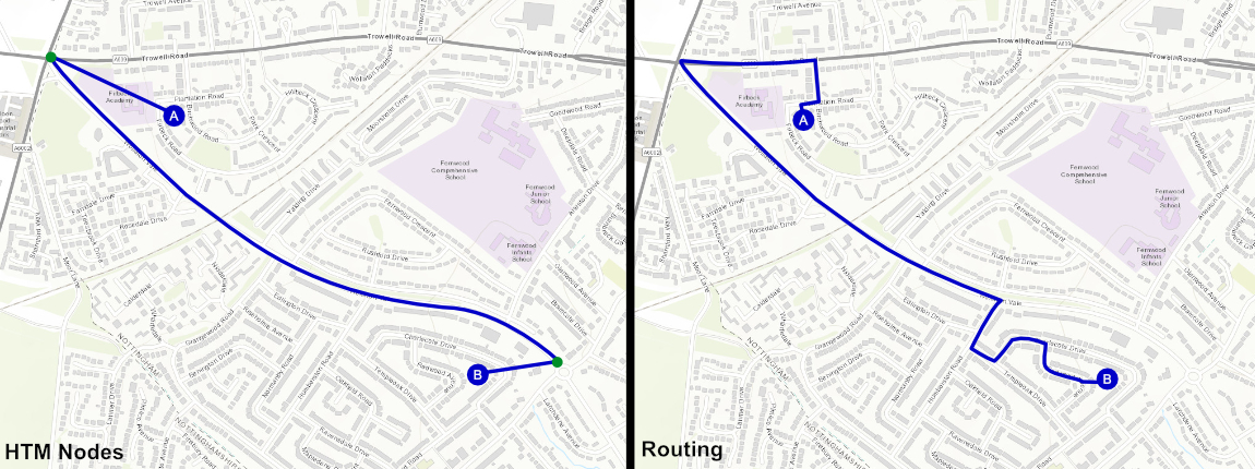
When calculating a travel, the straight line distance between the two locations is first calculated. If they are within a configured distance a routing calculation is done. This can be configured by the RoutingMaximumDistanceMeters parameter (Default: 4000 meters). Routing can be disabled by setting this parameter to 0.
To ensure good performance the routing calculation is stopped if the destination is not reached within a reasonable distance. If this happens the calculation falls back to a HTM calculation. This can be configured by the RoutingMaximumSearchMetersMultiplier parameter (Default: 2 [8000 meters]).
Warning
Routing parameters should not be altered unless advised to do so by IFS product development. Performance is affected by how fast the road network data can be loaded, how much memory is needed to hold the road network data and how many routes need to be calculated. The longer the travel distance the greater the calculation time needed, and the default values have been set to balance the performance cost against the improved travel estimation accuracy.
Routing Calculation Mode
Routing calculation has two modes of operation that can be controlled by the RoutingCalculator parameter (Default: TravelAnalyser).
- InProcess: The individual services that need routing calculations load and process the routing data in the same service. When processing a new LOAD the already loaded routing data is reloaded. When two different datasets use the same routing parameters the routing data is not shared.
- TravelAnalyser: The Scheduling Travel Analyser service handles routing calculations. This allows the routing data to be shared rather than loaded multiple times saving overall memory usage. When processing a new LOAD the already loaded routing data is reused. If two different datasets use the same routing parameters the routing data can be shared.
For the performance characteristics of the different routing calculation modes see the Architecture and Sizing Guide — Routing Calculation Mode.
Straight Line Travel
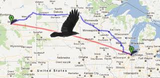
Straight Line Travel is a 'as the crow flies' travel calculation, i.e. the shortest distance between two points; the geodesic distance. While this is the shortest route possible, it is not representative of the real world as it doesn't take into consideration the routing network. However, for scheduling problems that travel accuracy is not of highest importance, e.g. travels that take a few hours, this travel option is often sufficient.
Real Time Travels
The Dynamic Scheduling Engine may be configured to use real time travel information from online routing services which includes up-to-date traffic information and possible road closures. Please contact IFS for details of available routing services.
Note
Real Time Travels are not a stand-alone travel solution. They serve as an additional travel accuracy option on top of existing travel options (HTM or Straight Line).
The additional accuracy of real time travel over the alternative travel calculation options (HierarchicalTravelMatrix and StraightLine) is of most benefit to imminent activities. To make best use of this we advise setting up a dedicated Profile which is configured for Committed activities and which uses the real time travel calculation method. The essential setup steps, which may be completed either by using system data input or the Scheduling Workbench Administration workspace, are:
- Add a Profile to be used by committed activities. For example, one with an ID of "CommittedActivitiesProfile" - you may leave the Description field blank.
- Set the "CommittedActivitiesProfileId" parameter to the ProfileId from the previous step, e.g. "CommittedActivitiesProfile". If using system data input, set the Profile for this parameter to your base profile, for example "DEFAULT".
- Set the "TravelCalculationOption" to "RealTimeTravel" with the ProfileId set consistent with the previous steps (i.e. "CommittedActivitiesProfile").
- Set the "RoutingApiKey" parameter. This is essential as the requests made to online routing services will typically require a valid API key.
- Set the "RealTimeTravelProvider" parameter. This identifies the real time travel provider: NONE, TOMTOM.
There are a number of additional parameters relating to real time travel calculations which can be set by the user, although their default values should suffice for most practical applications. These are:
- CommittedActivitiesProfileThreshold – defines the maximum time window (measured from the current schedule time) during which the CommittedActivitiesProfile is applied for activities with a committed-like status. For activities scheduled further in the future than this threshold, committed activities revert to using the default travel calculation option. With a configuration where the CommittedActivitiesProfile uses RealTimeTravel and the base profile uses a standard travel calculation method, such as HierarchicalTravelMatrix, this parameter allows you to tune how far ahead RealTimeTravel is considered. We recommend setting this threshold to a value that focuses on imminent work rather than distant activities, as applying RealTimeTravel too broadly can impact performance and unnecessarily process large volumes of activities. This is useful because traffic information for the distant future is often unnecessary.
- RealTimeTravelRefreshCacheFrequency - rate at which the real time travel information is refreshed. Smaller values mean more frequent refreshing of data at the cost of more requests to the online routing service which may impinge on performance.
- RealTimeTravelAvoidTolls - whether to avoid tolls in the real time travel route.
- RealTimeTravelAvoidHighways - whether to avoid highways/motorways in the real time travel route. Note: both RealTimeTravelAvoidTolls and RealTimeTravelAvoidHighways can be set simultaneously.
Note: although the RealTimeTravel option provides up-to-date travel information, it is not a practical option for use as the sole travel calculation method for an entire schedule. Therefore, we strongly advise that real time travels are used only for committed activities. For example, a suitable configuration would be to use real time travels for soon-to-be-commenced activities in combination with the Hierarchical Travel Matrix as the standard travel calculation problem.
Travel In A Resource's Shift
There are a number of ways of influencing the travel that a resource is able to carry out in a shift. These include:
- Travel before or after the shift.
- Travel limits.
- Adjustments to speed and calculation methods.
- Costs and penalties
- Travel part usage
Note
Attributes can be configured in the input data at three different levels: Resource Type, Resource and Shift. In each case the more specific level overrides, e.g. a value against a shift will override a value against a resource. For some attributes a default value for the entire dataset can also be specified via a database parameter. If the Advanced Resource Planner is being used then attributes can be set here and will be passed to the DSE.
Basic Travel Cost
Any travel in a resource's shift will incur both a time cost and a travel cost. The time cost comes from the cost per hour (or overtime cost per hour) associated to the shift, in exactly the same way as when the resource carries out activities.
The basic travel cost comes by default from the cost per km associated to the shift. Note however that if a travel cost model is used then the cost per km will be taken from this instead. The default value for the cost per km is 0.25, but this can be adjusted if required to discourage certain resources from having too much travel planned.
Note
Be aware that a high cost per km can have an unintended impact on the schedule, since it can make some activities not worth scheduling.
Travel Outside Shift Time
A resource can be set up to be expected to spend some time travelling either before the start of their shift, or after the end.
For example, suppose that a resource is due to start a shift at 9am, and is set to allow up to 45 minutes travel before the start of their shift. (This is known as travel to, since it is travel to the first activity). Then if the DSE planned an activity which was 30 minutes away the travel would be planned to start at 8:30am, with the resource arriving at 9am when the shift starts. If however the activity was 1 hour away then the resource would start travelling at 8:15am, and to arrive at 9:15am. This means that the resource is travelling for 45 minutes before the shift start (the maximum allowed time), plus another 15 minutes within the shift.
Note
By default the cost of this travel will be calculated as normal. However the time can also be made non-chargeable by setting the parameter 'TravelToAndFromChargeable' to false. Finally, more specific options can also be set by using the travel cost model.
Note
The fields 'travel_to' (travel at start of shift) and 'travel_from' (travel at end of shift) are used for this feature.
Maximum Travel
The business needs or rules may require that some limits are placed on how far a resource can travel. This restriction can be applied in three different ways:
- As a maximum radius from the shift start location.
- As a maximum travel time for each journey in a shift.
- As a maximum total travel time within a shift (only available via the travel cost model).
- As a maximum travel distance for each journey in a shift (only available via the travel cost model).
- As a maximum total travel distance for each journey in a shift (only available via the travel cost model).
If a travel cost model is used then each of these can be set independently, and also soft penalties can be set for exceeding limits instead of or as well as hard maximum values.
Otherwise the limit is set as a maximum travel time (via the 'max_travel' attribute). This attribute is always applied as a limit on how far the resource can travel from the shift start location. For example, if the maximum travel is set to half an hour, then the resource could be allocated an activity that is 29 mins away from the start location. However the DSE cannot schedule an activity that is 31 minutes away from the resource's start location (even if it is only two minutes away from the first activity in the resource's route).
By default the limit is also applied as a restriction on the travel time of each individual journey of the resource. For example, if the maximum travel is set to 30 mins, each individual journey (either to an activity or to/from start/end locations) must be below 30 mins.
Note
It is possible to turn off the second option by changing the DSE parameter 'MaxTravelAppliesToAllJourneys' to false. In this case the maximum travel will only be applied as a limit based on the shift start location.
Note
It is possible to violate this constraint, if an activity is fixed to a resource that has a travel time more than the max travel for the resource in that shift. In this case, the activity is scheduled as normal and an 'externally violated constraint' is raised called 'Activity fixed or committed to resource exceeding max travel';
Travel Cost Model
The travel cost model allows for more elaborate and comprehensive ways to configure travel cost. This includes:
- Soft penalties and incremental costs as well as hard limits on maximum travel.
- Limits on the total journey time within a shift.
- Fine control on the costs of travel before and after the shift.
- Applying additional time to journeys when exceeding a penalty threshold.
Please see the 'Travel Cost Model' section in the 'Costs and Values' guide for more detail.
Travel Settings
Often some resources have different travel circumstances than others. This could range from different speeds to entirely different methods of calculating travel time (e.g. different modes of transport).
As such, it is possible to link a resource (or indeed an individual shift) to a 'profile' from which any travel related parameter settings should be taken. These parameter settings include all in the parameter group 'TRAVEL', and in particular:
- TravelCalculationMethod - the method to use for travel calculation (e.g. HTM or straight line).
- HierarchicalDatabaseMatrixId - the id of the hierarchical travel matrix to use.
- LocationAddTime - additional time added for parking etc.
- SpeedFactor - acts as a multiplier on the journey time.
- TravelTimeProfileId - links to a travel time profile of travel weightings etc. See the section later in this guide.
Note
The field 'profile_id_travel' is used for this feature.
Speed Factor
A speed factor can also be set directly on resources and resource types. For example, a resource may drive a vehicle that is restricted to drive slower than normal vehicles, e.g. a large truck. A speed factor of 1.5 can then be set, which increases the expected journey time by 50%.
Note
The field 'speed_factor' is used for this feature.
Travel Part Usage
It is also possible to specify that parts should be consumed while travelling. This can be used to limit the amount of travel the resource can carry out, while also allowing for the part to be restocked via visits to activities and/or depots.
A typical use case for this would be to represent the range of an electric vehicle, with recharging points represented by depots. See the Parts concepts guide for further details.
Location Add Time
In many situations when a resource arrives at a particular activity location it may take some time for the resource to actually start working on the activity. This can be due to many reasons, such as the parking area is 10 mins walk from the actual location of the activity. If the user has this knowledge about certain activity locations a location add time can be linked to these locations.
Note
The field 'addtime' (add time) is used for this feature. The field is on all levels of locations: the Location Type entity and the Location entity. Please see the corresponding schema entity sections in the IFS Scheduling Schema Guide for more detail.
Travel Time Profiles
When the Dynamic Scheduling Engine calculates a travel time, it does this using certain parameters. These include whether to use straight line or a travel matrix, and various speed settings and additional times that can affect the calculation result.
One such parameter is named TravelTimeProfileId and it is this which determines which travel time profile is used.
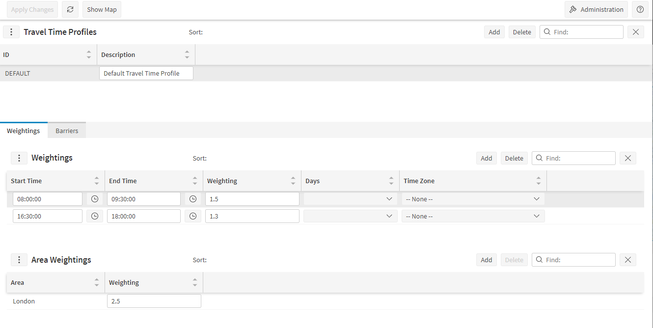
A travel time profile allows you to adjust the expected journey times used by the Dynamic Scheduling Engine, depending on the time of day and the area the journey covers.
It is possible to set up multiple travel time profiles, but initially the system will contain a single travel time profile named 'DEFAULT' which will be empty. Any changes to travel-related parameters are applied to all parameters that are linked to the 'DEFAULT' travel time profile by default (which should be all of the parameters if no other travel time profiles are set up). If you wish to use a travel time profile other than the default you simply set the value of this parameter to the travel time profile you wish to use.
There are two factors that make up the travel time profile:
- travel weightings
- travel barriers
Travel weightings allow you to specify a multiplier that should be applied to all travel journeys at a particular time of day and optionally in a particular area. There are three parts to this:
- Setting a multiplier (or weighting) that gets applied to all travels at particular times of day.
- Defining areas within which you wish to apply different weightings.
- Defining an override weighting for a particular area at a particular time of day.
Travel barriers allow you to specify where there are blockages within the travel network which will require a diversion to be taken and so add extra time to the journey.
Automated Intelligent Travel Profiles
Automated Intelligent Travel Profile (AITP) files are now optionally provided alongside the HTM database for customers to use. These files have been created from speed profile data generated by TomTom using advanced machine learning techniques. Each road segment is matched by TomTom to a speed profile which in turn gives an expected journey time for that road segment at any given time of day.
The AITP files are designed to complement HTMs and are expected to be produced alongside each new revision of the HTM. Urban areas (cities and larger towns) within the region covered by the HTM are automatically detected. For reference the North America AITP file includes just over 1000 urban areas, as shown below:
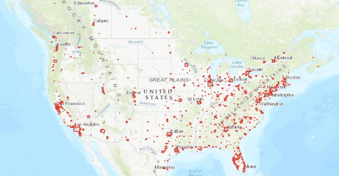
For each urban area a travel weighting is then calculated for each half hour period within typical working day hours (Monday-Friday 6am-8pm). This is done by comparing the normal expected journey time with the expected time when travelling at that specific time of day, using the TomTom speed profile data. This comparison is performed across several sets of test locations to ensure an accurate result.
These results are then converted into travel time weightings (including time zone information) to be used in conjunction with the HTM they accompany.
Note
There is an additional licence cost associated with the use of these files. See the Architecture and Sizing Guide for a list of currently available files.
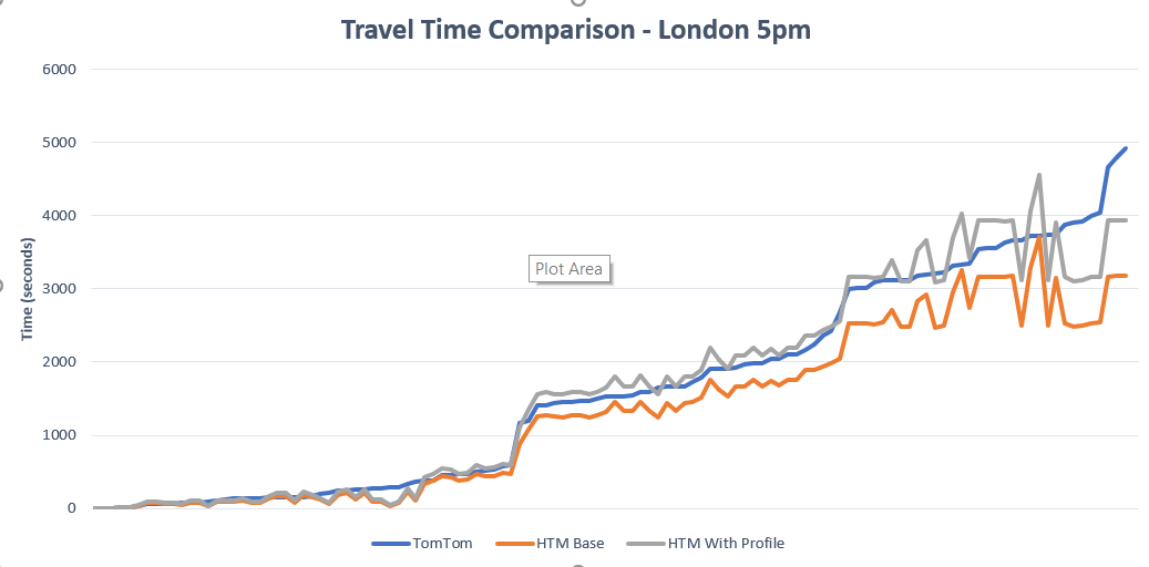
The improved accuracy in travel estimates can be seen in the comparison graph below, where the TomTom estimate (blue line) is compared to the HTM estimate both with (grey line) and without (orange line) the AITP travel time profile being applied. The overall journey time from the default HTM estimate is around 20% down at this time (which is to be expected given the rush hour), but with the travel profile applied there is less than 1% difference.
Note
The AITP files are .xml files that can be provided along with the HTM they accompany. These files can simply be imported into a PSO system via the 'Administration -> Import/Export -> System Data -> Import Data' option on the Scheduling Workbench.
This will add a single travel time profile with id matching the id of the HTM it accompanies. This can be viewed on the Scheduling Workbench via the 'Travel Time Profiles screen', and the urban areas covered can be viewed in the 'Area Editor'.
To begin using this travel time profile, the parameter 'TravelTimeProfileId' should be set to match the travel time profile id (which can be seen on the travel time profiles screen).
Note
Some customers may wish to import the AITP data into an existing travel time profile, for example because travel barriers are already set up in this profile. This can be done by editing the .xml file as follows:
- Remove the 'Travel_Time_Profile' row.
- Find and Replace
<travel_time_profile_id>{old id}</travel_time_profile_id>with<travel_time_profile_id>{new id}</travel_time_profile_id>where {old id} is the travel time profile id used in the file and {new id} is the id of the travel time profile you wish to import into. - Save the changes.
The file can then be imported as before.
It is strongly advised that you take an export of your current system data before doing this so that this can be restored again later if necessary. We also advise that you delete any existing weightings in this profile before importing the new data.
Weightings
It is also possible to set up custom travel time weightings (including area specific weightings) manually. This can be done using the 'Travel Time Profiles' screen in the Administration section of the Scheduling Workbench, and the process is described below.
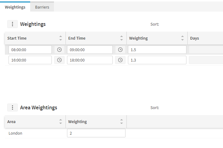
The top part of the screen is where you can define weightings that will apply to all travels at a particular time of day. In the example below we have defined two such weightings, one between 8am and 9am with a weighting of 1.5 and the other between 4pm and 6pm with a 1.3 weighting. (This would be to reflect the morning and afternoon rush hours).

The weighting is applied to any part of any journey falling within the specified times. The expected time taken to complete this part of the journey will be multiplied by the weighting value. So as a simple case a journey starting at 8:00am which would normally take 10 minutes will now take 15 minutes. For a journey starting at 8:45am and normally taking one hour, the total journey time will be increased to one hour and 5 minutes to reflect the fact that the first 15 minutes of the journey is in the morning rush period, where only 10 minutes of normal travel was possible.
It is also possible to create different weightings for specific days of the week within the same travel time profile using the Days column as shown below:
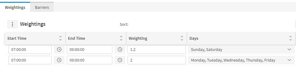
This means that within the same travel time profile you can specify two or more weightings which apply to different days of the week.
Finally you can also specify a time zone in which the weighting should be applied.

Note
Please note that if the time zone is not specified then the server time zone will be used when applying the weighting. This could lead to unexpected behaviour if the server time zone is not the same as the local time zone for the dataset.
Note
It is possible to set up several weightings each applying in different time zones. Please note however that the time zone specified will only affect the times at which the weighting is applied; it does not have any geographic impact. Therefore to ensure that a weighting only applies to a selected area the default weighting should be set to 1, and an area weighting should be used to specify the relevant area.
Areas
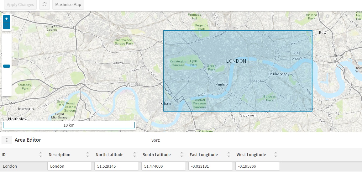
The travel time profile also allows you to define different weightings which apply only in certain areas. The first step to do this is to define the areas themselves, which is done using the area editor. In this example, we have defined a single area covering London.
Area Weightings
Once we have defined an area we can then define area weightings. These are applied within a particular weighting, and the weighting value specified will override the default value on the weighting itself. In the example below we have specified an override weighting of 2 for the London area in the morning rush hour, so travel in London between 8am and 9am will be expected to take twice as long as usual.
Note
This only applies within the morning rush hour - we can also specify an override value for the afternoon rush hour, which can if we like have a different weighting value.
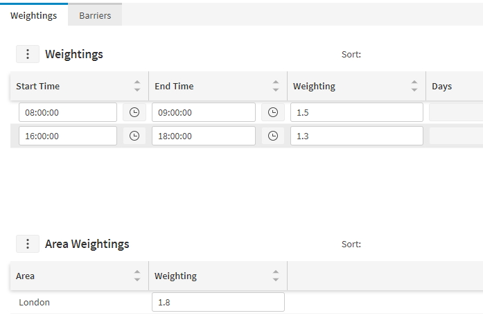
These area weightings will be applied to any part of any journey falling within the specified times and within the specified area. So a journey in London starting at 8:00am which would normally take 10 minutes will now take 20 minutes. If only part of the journey is in the London area then the default 1.5 weighting will be applied to the part of the journey not in the London area. The resulting journey time would therefore be somewhere between 15 and 20 minutes.
One special case to note is where a weighting is only required in a specified area. For example suppose we want to slow down all travel times in the London area only between 7am and 7pm. For this we simply specify the required times with a default weighting of 1 (so travels outside London will not be affected), and then set up our area weighting for London with the required weighting, say 1.5.
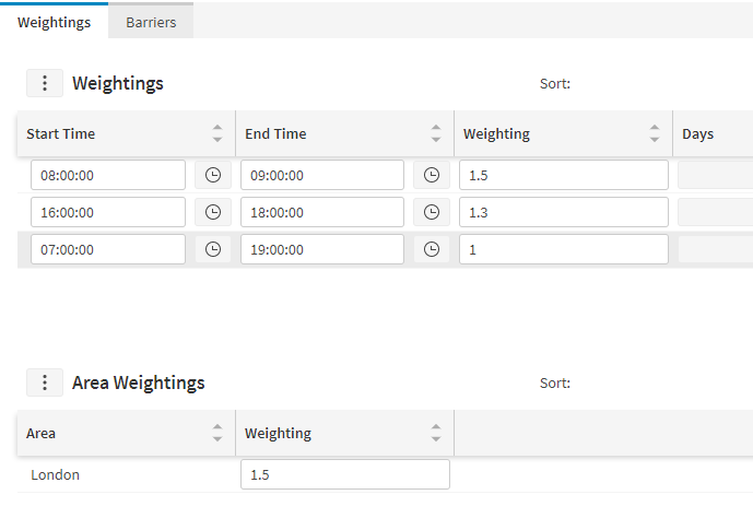
Note
The times specified in the weighting are allowed to overlap. If they do then the weighting from the smallest time interval will be applied, so in this case the weightings we defined earlier for the morning and afternoon rush periods will still be applied.
Barriers
A travel barrier can be used to add a delay to all journeys expected to cross a particular point on the travel network. There are several possible scenarios where this could be useful.
- Blocked roads. For example mountain roads that have been closed due to hazardous conditions.
- Avoiding additional costs. For example avoiding bridges where tolls are charged or avoiding ferry crossings.
- Avoiding crossing boundaries. For example to keep resources from crossing state boundaries.
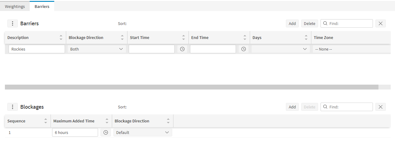
To create a travel barrier first choose a description in the top panel.
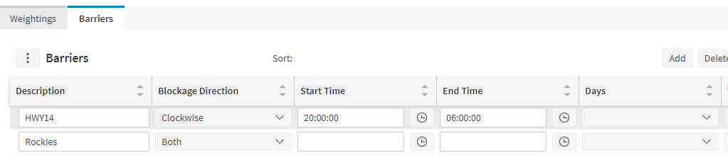
Optionally you can also restrict the barrier to apply only at certain times of day, and only on certain days of the week. If the blockage end time is set to earlier than the blockage start time, it will be assumed that the blockage applies overnight. If the barrier is restricted to certain times of day then you may also wish to specify a time zone to ensure that the time of day is applied correctly. If no time zone is specified then the times will be applied using the local server time zone.
Finally you can set the blockage direction. This defaults to 'Both', which means that the delay will affect all journeys that cross the barrier, regardless of the direction of travel. Blockages can also apply in only one direction, which is specified as either clockwise or anti-clockwise. Further details of this option are given later in this document.
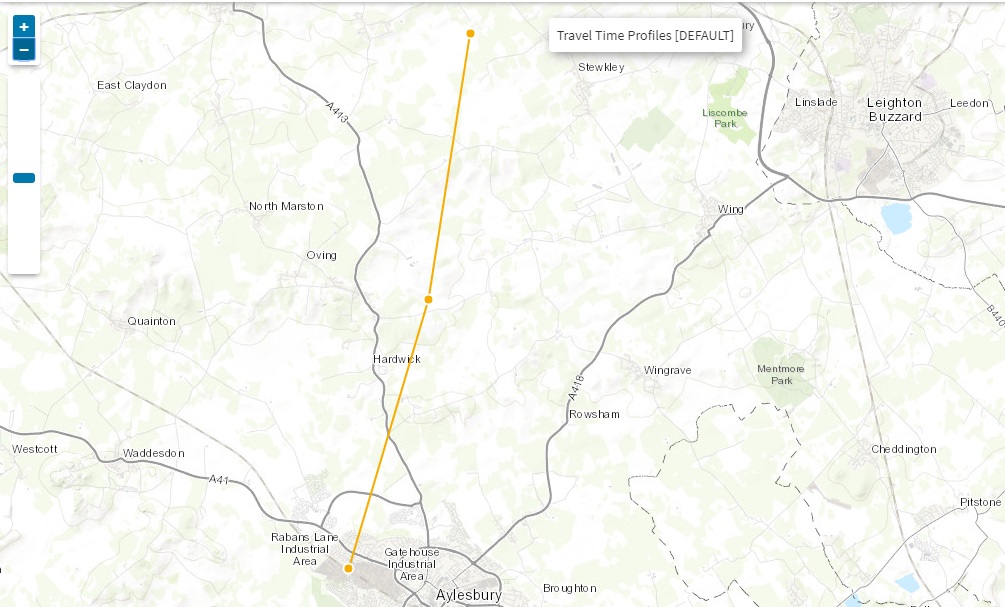
The barrier itself can then be created by clicking on the map. A double-click will create a new point on the barrier. Each point can then be dragged to a new position if required. Points can also be deleted by clicking the button in the top right of the right-hand panel.
When creating a barrier, please note the following:
- The start and end points of the barrier should be on the roads that can be used to divert around the barrier.
- A barrier point should be placed on all roads affected by the blockage.
- Points can also be placed where there are not roads in order to change the direction of the barrier. These points should not be marked as crossing points.
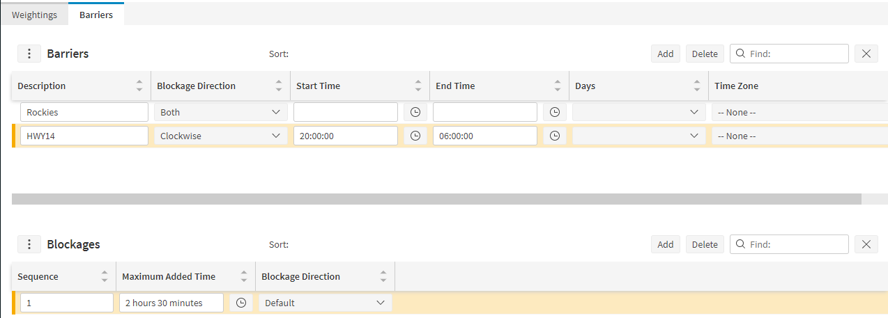
Finally it is necessary to define which points are blocked, and to set the blockage direction and maximum added time for each blocked point.
The maximum added time is the maximum time that will be added to a journey as a result of this blockage point. The value should be approximately the time taken to travel from one side of the blockage to the other, following the diversion.
The blockage direction is the direction in which the blockage applies. By default the blockage direction is taken from that specified on the barrier as a whole, but you can specify separate blockage directions for each blockage point. This could be that the blockage is in both directions, in one direction only (clockwise or anti-clockwise), or that this particular point on the barrier is clear (i.e. not blocked).
Note
To specify a one-way only blockage the blockage direction should be set to either 'clockwise' or 'anti-clockwise'. This is in relation to the line which defines the barrier.
A clockwise blockage means that the blockage will apply to all travels that cross the barrier travelling from the clockwise side. The clockwise side is the side defined by the arc between the lines from the previous barrier point to this point, and from this point to the next barrier point.
For example, suppose in the diagram below that there is a clockwise blockage at point 1.
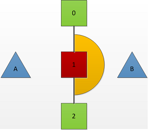
The clockwise side of the barrier is shown in orange. This starts from the line between point 0 and point 1. It then moves clockwise until it hits the line from point 1 to point 2.
As a result, journeys from B to A would be delayed by this blockage, but journeys from A to B would not.
Note
The actual time added to any journey will only be a proportion of the maximum added time specified. The proportion applied is calculated by comparing the straight line distances of a journey that goes via the crossing point with the same journey going via the nearest available diversion point.
For example, suppose a blockage point X and diversion point Y are 20km apart, with a maximum added time of 1 hour. Suppose a journey from points A to B crosses this barrier close to the blockage point X.
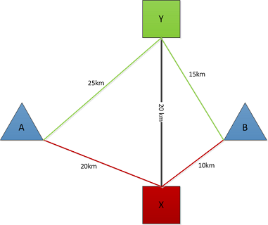
- The distance from A to point X is 20km, and from point X to B it is 10km, making a total distance of 30km.
- The distance from A to point Y is 25km, and from point Y to B it is 15km, making a total distance of 40km.
- It is therefore expected that the diversion will add around 10km to the journey.
- Since X and Y are 20km apart, the maximum added distance for any journey would be 40km.
- So for this journey the DSE will apply 10km/40km = 25% of the maximum added time - i.e. a 15 minute delay.